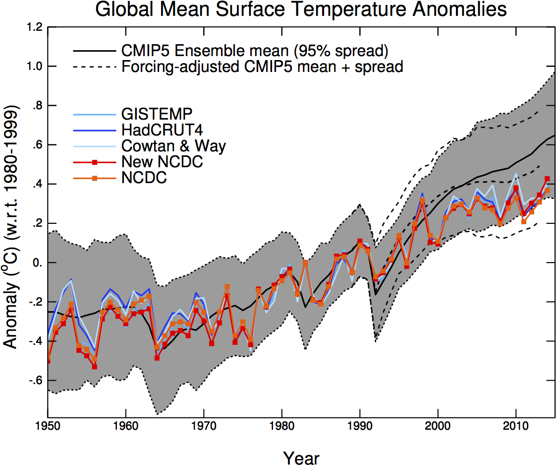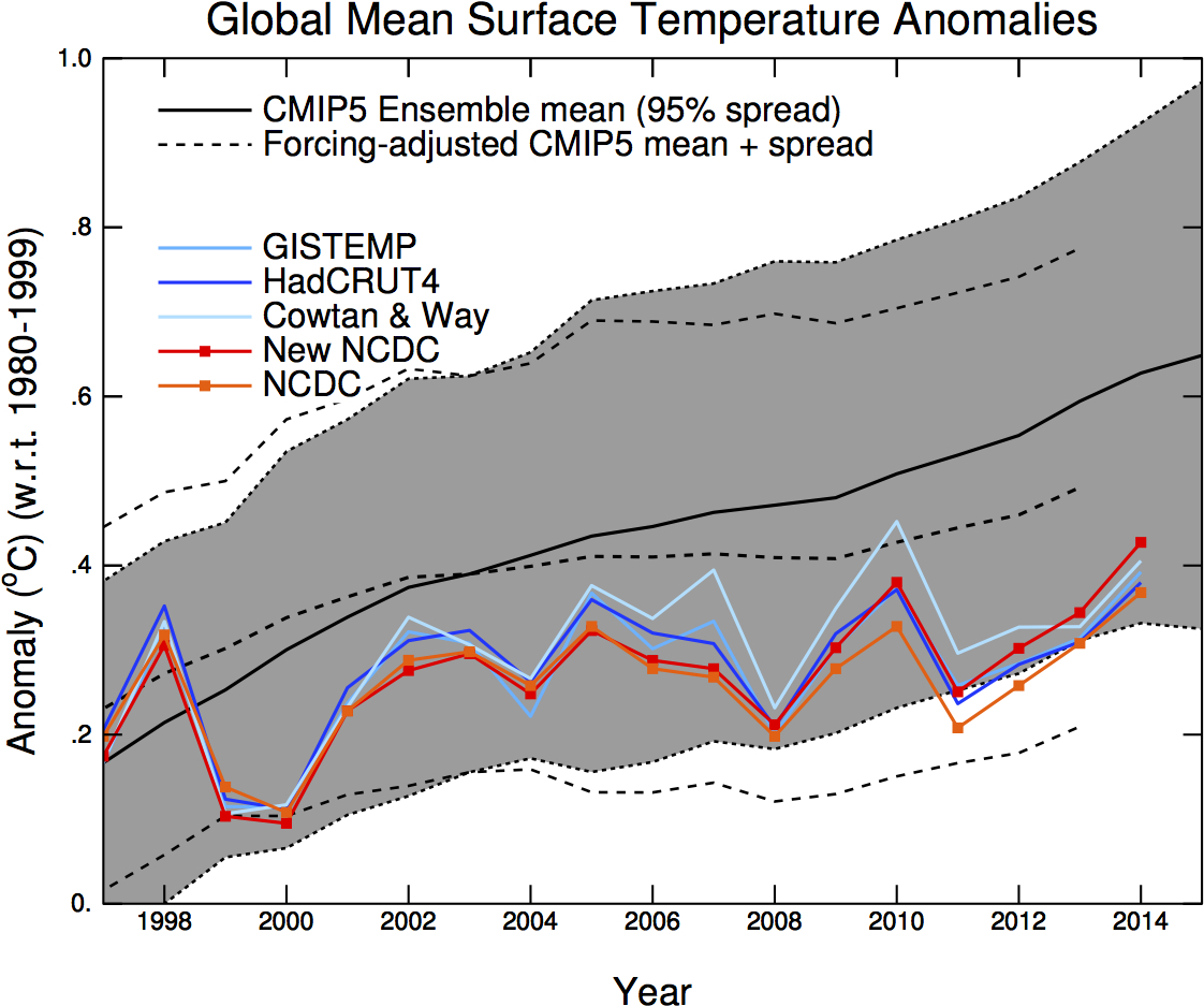
 Comparison of a large set of climate model runs (CMIP5) with several observational temperature estimates. The thick black line is the mean of all model runs. The grey region is its model spread. The dotted lines show the model mean and spread with new estimates of the climate forcings. The coloured lines are 5 different estimates of the global mean annual temperature from weather stations and sea surface temperature observations. Figures: Gavin Schmidt.
It seems as if 2015 and likely also 2016 will become very hot years. So hot that you no longer need statistics to see that there was no decrease in the rate of warming, you can easily see it by eye now. Maybe the graph also looks less deceptive now that the very prominent super El Nino year 1998 is clearly no longer the hottest.
The "debate" is therefore now shifting to the claim that "the models are running hot". This claim ignores the other main option: that the
observations are running cold. Even assuming the observations to be perfect, it is not that relevant that some years the observed annual mean temperatures were close to lower edge of the spread of all the climate model runs (ensemble spread). See
comparison shown at the top.
Now that we do not have this case for some years, it may be a neutral occasion to explain that the spread of all the climate model runs does
not equal the uncertainty of these model runs. Because also some scientists seem to make this mistake, I thought this was worthy of a post. One hint is naturally that the words are different. That is for a reason.
Long long ago at a debate at the scientific conference EGU there was an older scientist who was really upset by
ClimatePrediction.net, where the public can give their computer resources to produce a very large dataset with many different climate model runs with a range of settings for parameters we are uncertain about. He worried that the modeled distribution would be used as a statistical probability distribution. He was assured that everyone was well aware the model spread was not the uncertainty. But it seems he was right and this awareness has faded.

Ensemble weather prediction
It is easiest to explain this difference in the framework of ensemble weather prediction, rather than going to climate directly. Much more work has been done in this field (meteorology is bigger and decadal climate prediction has just started). Furthermore, daily weather predictions offer much more data to study how good the prediction was and how good the ensemble spread fits to the uncertainty.
While it is popular to complain about weather predictions, they are quite good and continually improving. The prediction for 3 days ahead is now as good as the prediction for the next day when I was young. If people really thought the weather prediction was bad, you have to wonder why they pay attention to it. I guess, complaining about the weather and predictions is just a save conversation topic. Except when you stumble upon a meteorologist.
Part of the recent improvement of the weather predictions is that not just one, but a large number of predictions is computed, what scientists call: ensemble weather prediction. Not only is the mean of such an ensemble more accurate than just the single realization we used to have, the ensemble spread also gives you an idea of the uncertainty of the prediction.
Somewhere in the sunny middle of a large high-pressure system you can be quite confident that the prediction is right; errors in the position of the high are then not that important. If this is combined with a blocking situation, where the highs and lows do not move eastwards much, it may be possible to make very confident predictions many days in advance. If a front is approaching it becomes harder to tell well in advance whether it will pass your region or miss it. If the weather will be showery, it is very hard to tell where exactly the showers will hit.
Ensembles give information on how predictable the weather is, but they do not provide reliable quantitative information on the uncertainties. Typically the ensemble is overconfident, the ensemble spread is smaller than the real uncertainty. You can test this by comparing predictions with many observation. In the figure below you can read that if the raw model ensemble (black line) is 100% certain (forecast probability) that it will rain more than 1mm/hr, it should only have been 50% sure. Or when 50% of the model ensemble showed rain, the observations showed 30% of such cases.
 The "reliability diagram" for an ensemble of the regional weather prediction system of the German weather service for the probability of more than 1 mm of rain per hour. On the x-axis is the probability of the model, on the y-axis the observed frequency. The thick black line is the raw model ensemble. Thus when all ensemble members (100% probability) showed more than 1mm/hr, it was only rain that hard half the time. The light lines show results two methods to reduce the overconfidence of the model ensemble. Figure 7a from Ben Bouallègue et al. (2013).
To generate this "raw" regional model ensemble, four different global models were used for the state of the weather at the borders of this regional weather prediction model, the initial conditions of the regional atmosphere were varied and different model configurations were used.
The raw ensemble is still overconfident because the initial conditions are given by the best estimate of the state of the atmosphere, which has less variability than the actual state. The atmospheric circulation varies on spatial scales of millimeters to the size of the planet. Weather prediction models cannot model this completely, the computers are not big enough, rather they compute the circulation using a large number of grid boxes with are typically 1 to 25 km in size. The flows on smaller scales do influence the larger scale flow, this influence is computed with a strongly simplified model for turbulence: so called parameterizations. These parameterization are based on measurements or more detailed models. Typically, they aim to predict the mean influence of the turbulence, but the small-scale flow is not always the same and would have varied if it would have been possible to compute it explicitly. This variability is missing.
The same goes for the parameterizations for clouds, their water content and cloud cover. The cloud cover is a function of the relative humidity. If you look at the data, this relationship is very noisy, but the parameterization only takes the best guess. The parameterization for solar radiation takes these clouds in the various model layers and makes assumptions how they overlap from layer to layer. In the model this is always the same; in reality it varies. The same goes for precipitation, for the influence of the vegetation, for the roughness of the surface and so on. Scientists have started working on developing parameterizations that also simulate the variations, but this field is still in its infancy.
Also the data for the boundary conditions (height and roughness of the vegetation), the brightness of the vegetation and soil, the ozone concentrations and the amount of dust particles in the air (aerosols) are normally taken to be constant.
For the raw data fetishists out there: Part of this improvement in weather predictions is due to the statistical post processing of the raw model output. From simple to complicated: it may be seen in the observations that a model is on average 1 degree too cold, it may be known that this is two degrees for a certain region, this may be due to biases especially during sunny high-pressure conditions. The statistical processing of weather predictions to reduce such known biases is known as model output statistics (MOS). (This is methodologically very similar to the
homogenization of daily climate data.)
The same statistical post-processing for the average can also be used to correct the overconfidence of the model spread of the weather prediction ensembles. Again from the simple to the complicated. When the above model ensemble is 100% sure it will rain, this can be corrected to 50%. The next step is to make this correction dependent on the rain rate; when all ensemble members show strong precipitation, the probability of precipitation is larger than when most only show drizzle.
Climate projection and prediction
There is no reason whatsoever to think that the model spread of an ensemble of climate projections is an accurate estimate of the uncertainty. My inexpert opinion would be that for temperature the spread is likely again too small, I would guess up to a factor two. The better informed authors of the last IPCC report seems to agree with me when
they write:
The CMIP3 and CMIP5 projections are ensembles of opportunity, and it is explicitly recognized that there are sources of uncertainty not simulated by the models. Evidence of this can be seen by comparing the Rowlands et al. (2012) projections for the A1B scenario, which were obtained using a very large ensemble in which the physics parameterizations were perturbed in a single climate model, with the corresponding raw multi-model CMIP3 projections. The former exhibit a substantially larger likely range than the latter. A pragmatic approach to addressing this issue, which was used in the AR4 and is also used in Chapter 12, is to consider the 5 to 95% CMIP3/5 range as a ‘likely’ rather than ‘very likely’ range.
The confidence interval of the "very likely" range is normally about twice as large as the "likely" range.
The ensemble of climate projections is intended to estimate the long-term changes in the climate. It was never intended to be used on the short term. Scientists have just started doing that under the header of "decadal climate prediction" and that is hard. That is hard because then we need to model the influence of internal variability of the climate system, variations in the oceans, ice cover, vegetation and hydrology. Many of these influences are local. Local and short term variation that are not important for long-term projections of global means thus need to be accurate for decadal predictions. The to be predicted variations in the global mean temperature are small; that we can do this at all is probably because regionally the variations are larger. Peru and Australia see a clear influence of El Nino, which makes it easier to study. While El Nino is the biggest climate mode, globally its effect is just a (few) tenth of a degree Celsius.
Another interesting climate mode is the [[
Quasi Biannual Oscillation]] (QBO), an oscillation in the wind direction in the stratosphere. If you do not know it, no problem, that is one for the climate mode connoisseur. To model it with a global climate model, you need a model with a very high top (about 100 km) and many model layers in stratosphere. That takes a lot of computational resources and there is no indication that the QBO is important for long-term warming. Thus naturally most, if not all, global climate model projections ignore it.
Ed Hawkins has a post showing the internal variability of a large number of climate models. I love the name of the post:
Variable Variability. It shows the figure below. How variable the variability between models is shows how much effort modellers put into modelling internal variability. For that reason alone, I see no reason to simply equate the model ensemble spread with the uncertainty.

Natural variability
Next to the internal variability there is also natural variability due to volcanoes and solar variations. Natural variability has always been an important part of climate research. The CLIVAR (climate variability and predictability) program is a component of the World Climate Research Programme and
its predecessor started in 1985. Even if in 2015 and 2016, the journal Nature will probably publish less "hiatus" papers, natural variability will certainly stay an important topic for climate journals.
The studies that sought to explain the "hiatus" are still useful to understand why the temperatures were lower some years than they otherwise would have been. At least the studies that hold; I am not fully convinced yet that the data is good enough to study such minute details. In the
Karl et al. (2015) study we have seen that small updates and reasonable data processing differences can produce small changes in the short-term temperature trends that are, however, large relative to something as minute as this "hiatus" thingy.
One reason the study of natural variability will continue is that we need this for decadal climate prediction. This new field aims to predict how the climate will change in the coming years, which is important for impact studies and prioritizing adaptation measures. It is hoped that by starting climate models with the current state of the ocean, ice cover, vegetation, chemistry and hydrology, we will be able to make regional predictions of natural variability for the coming years. The confidence intervals will be large, but given the large costs of the impacts and adaptation measures, any skill has large economic benefits. In some regions such predictions work reasonably well. For Europe they seem to be very challenging.
This is not only challenging from a modelling perspective, but also puts much higher demands on the quality and regional detail of the climate data. Researchers in our German decadal climate prediction project, MiKlip, showed that the differences between the different model systems could only be assessed well using a
well homogenized radiosonde dataset over Germany.
Hopefully, the research on decadal climate prediction will give scientists a better idea of the relationship between model spread and uncertainty. The figure below shows a prediction from the last IPCC report, the hatched red shape. While this is not visually obvious, this uncertainty is much larger than the model spread. The likelihood to stay in the shape is 66%, while the model spread shown covers 95% of the model runs. Had the red shape also shown the 95% level, it would have been about twice as high. How much larger the uncertainty is than the model spread is currently to a large part expert judgement. If we can formally compute this, we will have understood the climate system a little bit better again.

Related reading
In a blind test, economists reject the notion of a global warming pause
Are climate models running hot or observations running cold?
Reference
Ben Bouallègue, Zied, Theis, Susanne E., Gebhardt, Christoph, 2013:
Enhancing COSMO-DE ensemble forecasts by inexpensive techniques.
Meteorologische Zeitschrift,
22, p. 49 - 59, doi:
10.1127/0941-2948/2013/0374.
Rowlands, Daniel J., David J. Frame, Duncan Ackerley, Tolu Aina, Ben B. B. Booth, Carl Christensen, Matthew Collins, Nicholas Faull, Chris E. Forest, Benjamin S. Grandey, Edward Gryspeerdt, Eleanor J. Highwood, William J. Ingram, Sylvia Knight, Ana Lopez, Neil Massey, Frances McNamara, Nicolai Meinshausen, Claudio Piani, Suzanne M. Rosier, Benjamin M. Sanderson, Leonard A. Smith, Dáithí A. Stone, Milo Thurston, Kuniko Yamazaki, Y. Hiro Yamazaki & Myles R. Allen, 2012:
Broad range of 2050 warming from an observationally constrained large climate model ensemble. Nature Geoscience,
5, pp. 256–260, doi:
10.1038/ngeo1430.


