Trend errors in raw temperature station data due to inhomogeneities

Another serious title to signal this is again one for the nerds. How large is the uncertainty in the temperature trends of raw station data due to inhomogeneities? Too Long, Didn’t Read: they are big and larger in America than in Germany.

We came up with two very different methods (Lindau and Venema, 2020) to estimate this and we got lucky: the estimates match as well as one could expect.

Direct method

Let’s start simple, take pairs of stations and compute their difference time series, that is, we calculate the difference between two raw temperature time series. For each of these difference series you compute the trend and from all these trends you compute the variance.

If you compute these variances for pairs of stations in a range of distance classes you get the thick curves in the figure below for the United States of America (marked as U) and Germany (marked as G). This was computed based on data for the period 1901 to 2000 from the International Surface Temperature Initiative (ISTI) .

Figure 1. The variance of the trend differences computed from temperature data from the United States of America (U) and for Germany (G). Only the thick curves are relevant for this blog post and are used to compute the trend uncertainty. The paper used Kelvin [K], we could also have used degree Celsius [°C] like we do in this post.

When the distance between the pairs is small (near zero on the x-axis) the trend differences are mostly due to inhomogeneities, whereas when the distances get larger also real climate trend differences increase the variance of the trend differences. So we need to extrapolate the thick curves to a distance of zero to get the variance due to inhomogeneities.

For the USA this extrapolation gives about 1 °C² per century². This is the variance due to two stations. If the inhomogeneities are assumed to be independent, one station will have contributed half and the trend variance of one station is 0.5 °C² per century². To get an uncertainty measure that is easier to understand for humans, you can take the square root, which gives the standard deviation of the trends: 0.71 °C per century.

That is a decent size compared to the total warming over the last century of about 1.5 °C over land; see estimates below. This alone is a good reason to homogenize climate data to reduce such errors.

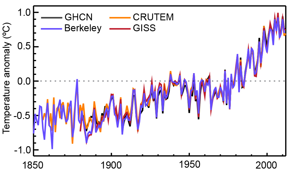
Figure 2. Warming estimates of the land surface air temperature from four different institutions. Figure taken from the last IPCC report.

The same exercise for Germany estimates the variance to be 0.5 °C² per century², the square root of half this variance gives a trend uncertainty of 0.5 °C per century.

In Germany the maximum distance for which we have a sufficient number of pairs (900 km) is naturally smaller than for America (over 1200 km). Interestingly, for America also real trend differences are important, which you can see in the trend variance increasing for pairs of stations that are further apart. In Germany this does not seem to happen even for the largest distances we could compute.

An important reason to homogenize climate data is to remove network-wide trend biases. When these trend biases are due to changes that affected all stations, they will hardly be visible in the difference time series. A good example is a change of the instruments affecting an entire observational network. It is also possible to have such large-scale trend biases due to rare, but big events, such as stations relocating from cities to airports, leading to a greatly reduced urban heat island effect. In such a case, the trend difference would be visible in the difference series and would thus be noticed by the above direct method.

Indirect method

The indirect method to estimate the station trend errors starts with an estimate of the statistical properties of the inhomogeneities and derives a relationship between these properties and the trend error.

Inhomogeneities

How the statistical properties of the inhomogeneities are estimated is described in Lindau and Venema (2019) and my previous blog post. To summarize, we had two statistical models for inhomogeneities. One where the size of the inhomogeneity between two breaks is given by a random number. We called this Random Deviations (RD) from a baseline. The second model is for breaks behaving like Brownian Motion (BM). Here the jump sizes are determined by random numbers. So the difference is whether the levels or the jumps are random numbers.

We found in both countries RD break with a typical jump size of about 0.5 °C. But the frequency was quite different, while in Germany we had one break every 24 years, in America it was once every 5.8 years.

Furthermore, in America there are also breaks that behave like Brownian Motion. For these break we only know the variance of the break multiplied by the frequency of the breaks, this is 0.45 °C² per century². We do not know not whether the value is due to many small breaks or one big one.

Relationship to trend errors

The next step is to relate these properties of the inhomogeneities to trend errors.

For the Random Deviation case, the dependence on the size of the breaks is trivial, it is simply proportional, but the dependence on the number of breaks is quite interesting. The numerical relationship is shown with +-symbols in the graph below.

Clearly when there are no breaks, there is also no trend error. On the other extreme of a large number of breaks, the error is due to a large number of independent random numbers, which to a large part cancel each other out. The largest trend errors are thus found for a moderate number of breaks.

To understand the result we start with the case without any variations in the break frequency. That is, if the break frequency is 5 breaks per century, every single 100-year time series has exactly 5 breaks. For this case we can derive an equation shown below as the thick curve. As expected it starts at zero and the maximum trend error is in case of 2 breaks in the time series.

More realistic is the case when there is a mean break frequency over all stations, but the number of breaks varies randomly per station. In case the breaks are independent of each other one would expect the number of breaks to follow a Poisson distribution. The thin lines in the graph below takes this scatter into account by computing a weighted average over the equation using Poisson weights. This smoothing reduces the height of the maximum and shifts it to a larger average break frequency, about 3 breaks per time series. Especially for more than 5 breaks, the numerical and analytical solutions fit very well.

Figure 3. The relationship between the variance of the trend due to inhomogeneities and the frequency of breaks, expressed as breaks per century. The plus-symbols are the results based on numerical simulation for 100-years time series. The thick line is the equation we found for a fixed break frequency, while the thin line takes into account random variations in the break frequency.

The next graph, shown below, also includes the case of Brownian Motion (BM), as well as the Random Deviation (RD) case. To make the BM and RD cases comparable, they both have jumps following a normal distribution with a variance of 1 °C². Clearly the Brownian Motion case (with O-symbols) produces much larger trend errors than the Random Deviations case (+-symbols).

Figure 4. The variance of the trend as a function of the frequency of breaks for the two statistical models. The O-symbols are for Brownian Motion, the +-symbols for Random Deviations. The variance of the jump sizes was 1 °C² in both cases.

That the variance of the trends due to inhomogeneities is a linear function of the number of breaks can be understood by considering that to a first approximation the trend error for Brownian Motion is given by a line connecting the first and the last segment of the break signal. If k is the number of breaks, the value of the last segment is the sum of k random values. Thus if the variance of one break is σ_β², the variance of the value of the last segment is k*σ_β² and thus a linear function of the number of breaks.

Alternatively you can do a lot of math and at the end find that the problem simplifies like a high school problem and that the actual trend error is 6/5 times the simple approximation from the previous paragraph.

Give me numbers

The variance of the trend error due to BM inhomogeneities in America is thus 6/5 times 0.45 °C² per century², which equals 0.54 °C² per century².

This BM trend error is a lot bigger than the trend error due to the RD inhomogeneities, which for 17.1 breaks per century and a break size distribution with variance 0.12 °C² is 0.13 °C² per century².

One can add these two variances together to get 0.67 °C² per century². The standard deviation of this trend error is thus quite big: 0.82 °C per century and mostly due to the BM component.

In Germany, we found only RD breaks with a frequency of 4.1 breaks per century. Their size is 0.13 °C². If we put this into the equation, the variance of the trends due to inhomogeneities is 0.34 °C² per century². Although the size of the RD breaks is about the same as in America, their influence on the station trend errors is larger, which is somewhat counter-intuitively because their number is lower. The standard deviation of the trend due to inhomogeneities is thus 0.58 °C per century in Germany.

Comparing the two estimates

Finally, we can compare the direct and indirect estimates of the trend errors. For America the direct (empirical) method found a trend error of 0.71 °C per century and the indirect (analytical) method 0.82 °C per century. For Germany the direct method found 0.5 °C per century and the indirect method 0.58 °C per century.

The indirect method thus found slightly larger uncertainties. Our estimates were based on the assumption of random station trend errors, which do not produce a bias in the trend. A difference in sensitivity to such biasing inhomogeneities in the observational data would be a reasonable explanation for these small differences. Also missing data may play a role.

Inhomogeneities can be very complicated. The break frequency does not have to be constant, the break sizes could depend on the year. Random Deviations and Brownian Motion are idealizations. In that light, it is encouraging that the direct and indirect estimates fit that well. These approximations seem to be sufficiently realistic, at least for the computation of station trend errors.

Variable Variability

Pages

Sunday 1 March 2020