A short introduction to the time of observation bias and its correction

Figure 1. A thermo-hygrograph, measures and records temperature and humidity.

Due to recent events, the time of observation bias in climatological temperature measurements has become a hot topic. What is it, why is it important, why should we and how can we correct for it? A short introduction.

Mean temperature

The mean daily temperature can be determined in multiple ways. Nowadays, it is easy to measure the temperature frequently, store it in a digital memory and compute the daily average. Also in the past something similar was possible using a thermograph; see Figure 1. However, such an instrument was expensive and fragile.

Thus normally other ways were used for standard measurements, using minimum and maximum thermometers and by computing a weighted average over observations at 3 or 4 fixed times. Another good approximation for many climate regions is to average over the minimum and maximum temperature. Special minimum and maximum thermometers were invented in 1782 for this task.

Not in every climate region the minimum and maximum temperature are well suited. For example in Iceland (part 1, part 2), the diurnal temperature range is small compared to the natural day to day (synoptic) variability. In such a case, fixed hour measurements are preferred. Fixed hour measurements are also performed for meteorological purposes. Four times a day, meteorologists all over the world make measurements, at the same time: 0, 6, 12 and 18 hour universal time (UTC).

Measuring four times a day is no fun, you have to get up at night, every night. Thus often the so-called Mannheimer hours (German Wikipedia) are used: 7, 14 and 21 hour local time; to compute the daily mean temperature, the measurement at 21 hours get a double weight.

In general, minimum and maximum temperature measurements are performed at voluntary climatological stations, whereas professional meteorological stations also perform fixed hour observations. Nowadays more and more stations are converted in automatic weather stations to save labour costs, which is an important change in the statistical properties of daily temperature records.

Time of observation bias

Naturally you can get a time of observation bias with the fixed hour measurements and changing these hours could thus produce a jump in a climatic temperature record. How large this jump would be could be determined by performing hourly measurements.

Mostly, the term time of observation bias (TOB), however, refers to minimum and maximum temperature measurements. At first glance, one might not expect any problem here. However, there are two reasons. If a thermometer is read before 24 hour, this means that partially the previous day is involved. And in case of monthly averages that a few hours of the previous month are included in this mean. This small temporal drift can make a difference, especially in spring and autumn.

A second bias may occur if the maximum temperature is read close to the typical maximum of the day or if the minimum temperature is read close to the time of the minimum temperature. If, for example, one night is exceptionally cold and the thermometer is read in the morning and then reset for the next day, the minimum temperature of that next day may be the same cold night. Such events may thus be counted double. The same can happen in reverse to the maximum temperature readings around noon. Typical errors for the USA are shown by the stripped curve in Figure 2.

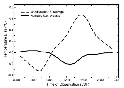Figure 2. Temperature bias over the day before and after correction, from Vose et al. (2003).

Correction of the TOB

The corrections for the TOB are here explained using the method of the NOAA as example (Vose et al., 2003). In the cooperative Network the observations are taken at an hour that is convenient for the volunteer observer (DeGaetano, 2000). It can change when the observer changes or when the observer preference changes.

The correction for the slightly different period can be corrected using a simple linear function including the observation time and the temperature difference between the current and the previous month (Karl et al. 1986).

The bias due to double counting of exceptionally cold or warm days depends on the local weather (diurnal cycle and synoptic variability). To derive this correction, hourly measurements are needed. (Subhourly measurements are only a little more precise.) This is only available for some stations, in the USA for about 500 stations. For these stations the correction can be computed for every possible "reading hour". To be able to correct the stations, which only have daily observations, a simple equation is derived (multiple linear regression) in which the monthly TOB bias correction is a function of the station coordinates (time zone, latitude and longitude), observation hour, average diurnal temperature range and average day-to-day temperature difference (Karl et al. 1986).

The performance of this correction can be tested on the 500 stations for which hourly measurements are available. (For the statisticians: The correction function was derived using data from 1957 to 1964, the errors in Figure 2 have been computed using independent data from 1965 to 2001.) The correction clearly makes the time of observation bias smaller. The largest errors are for readings taken just after noon, but as Figure 3 below shows, during this time period only small part of the readings are performed. The measurements performed at 00 hours account for about 10% of all readings and are mainly from more urban stations staffed by the Nation Weather Service, which are staffed 24 hours (DeGaetano, 2000).

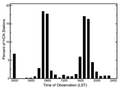Figure 3. Histogram of times the thermometers are read, Vose et al. (2003).

Homogenisation

Looking at Figure 2, a change in observation time can easily make a difference of up to 1°C. And the effect is even larger in winter when the diurnal cycle is smaller and double counting consequently happens more often. A bias in itself is no problem for studying trends in large climatic regions as long as it does not change. However, in the USA there is a tendency to morning observations. In the beginning of the network, the Weather Bureau recommended reading during sunset (Karl et al., 1986). Whereas in modern times more and more volunteers combine temperature observations with precipitation observations needed for flood forecasting; precipitation observations are performed in the morning. From the 1930s to 1990s the percentage of Historical Climate Network (HCN) stations reporting simultaneous precipitation and temperature observations (and thus reading in the morning) has increased from 56% to over 88% (DeGaetano, 2000). Without a TOB correction this would lead to an artificial climate trend.

The time of observation is nowadays known for every station and month, but especially in the beginning of the HCN (before 1950) this information is often missing, which limits the use of this data. Furthermore, this data (metadata: data about the data) can be wrong. It should thus be reminded that the correction of the TOB is only one part of the homogenization procedure. In homogenization first all known inhomogeneities are corrected. This can be the TOB correction, but also breaks for which the size is known from parallel measurements with the old and new set-ups over several years.

After these physical corrections, statistical homogenisation is applied. If the TOB correction was not accurate or the information on the observation times was wrong, there may be a jump in the data after the TOB correction. This can be removed in the statistical homogenisation step, in which every station is compared with its neighbours, in the USA using the pairwise homogenisation algorithm (PHA). (Many other homogenisation algorithm are also available on the web.) This step aims to remove all remaining inhomogeneities, not only the ones due to TOB. I have previously written about statistical homogenisation in more detail. The most used and most advanced algorithms have been validated in a blind benchmarking test. It was found that statistical homogenisation, even without the use of meta-data (known breaks and break sizes), improves the quality of temperature data and does not lead to spurious trends.

More posts on homogenisation

Statistical homogenisation for dummies

A primer on statistical homogenisation with many pictures.

Homogenisation of monthly and annual data from surface stations

A short description of the causes of inhomogeneities in climate data (non-climatic variability) and how to remove it using the relative homogenisation approach.

New article: Benchmarking homogenisation algorithms for monthly data

Raw climate records contain changes due to non-climatic factors, such as relocations of stations or changes in instrumentation. This post introduces an article that tested how well such non-climatic factors can be removed.

HUME: Homogenisation, Uncertainty Measures and Extreme weather

Proposal for future research in homogenisation of climate network data.

External link

As the TOB problem is especially important in the USA, people interested in this post may be interested in how the US Historical Climate Network data is processed.

References

Degaetano, A.T. A Serially Complete Simulated Observation Time Metadata File for U.S. Daily Historical Climatology Network Stations. Bulletin of the American Meteorological Society, 81, Issue 1, pp.49-68, doi: 10.1175/1520-0477(2000)081<0049:ASCSOT>2.3.CO;2, 2000.

Karl, T.R., C.N. Williams Jr., P.J. Young, W.M. Wendland. A Model to Estimate the Time of Observation Bias Associated with Monthly Mean Maximum, Minimum and Mean Temperatures for the United States. Journal of Applied Meteorology, 25, Issue 2, pp.145-160, doi: 10.1175/1520-0450(1986)025<0145:AMTETT>2.0.CO;2, 1986.

Russell S. Vose, Claude N. Williams Jr., Thomas C. Peterson, Thomas R. Karl, and David R. Easterling. An evaluation of the time of observation bias adjustment in the U.S. Historical Climatology Network. Geophys. Res. Lett., 30, no. 20, 2046, doi: 10.1029/2003GL018111, 2003.

Also see Ari's page on time of observations papers.