The fight for the future of science in Berlin

A group of scientists, scholars, data scientists, publishers and librarians gathered in Berlin to talk about the future of research communication. With the scientific literature being so central to science, one could also say the conference was about the future of science.

This future will be more open, transparent, findable, accessible, interoperable and reusable.


The open world of research from Mark Hooper on Vimeo.

Open and transparent sounds nice and most seem to assume that more is better. But it can also be oppressive, help the powerful with the resources to mine the information efficiently.

This is best known when it comes to government surveillance, which can be dangerous; states are powerful and responsible for the biggest atrocities in history. The right to vote in secret, to privacy, to organize and protections against unreasonable searches are fundamental protections against power abuse.

Powerful lobbies and political activists abuse transparency laws to harass inconvenient science.

ResearchGate, Google Scholar profiles and your ORCID ID page contribute to squeezing scientists like lemons by prominently displaying the number of publications and citations. This continual pressure can lead to burnout, less creativity and less risk taking. It encourages scientists to pick low hanging fruits rather than do those studies they think would bring science forward the most. Next to this bad influence on publications many other activities, which are just as important for science, suffer from this pressure. Many good-willing people were trying to solve this by also quantifying these activities. But in doing so add more lemon presses.


That technology brings more surveillance and detrimental micro-management is not unique to science. The destruction of autonomy is a social trend, that, for example, also affects truckers.

Science is a creative profession (even if many scientists do not seem to realise this). You have good ideas when you relax under the shower, in bed with fever or on a hike. The modern publish or perish system is detrimental to cognitive work. Work that requires cognitive skills is performed worse if you pressure people, it needs autonomy, mastery and purpose.

Scientists work on the edge of what is known and invariably make mistakes often. If you are not making mistakes you are not pushing your limits. This needs some privacy because unfortunately making mistakes is not socially acceptable for adults.

Chinese calligraphy with water on a stone floor. More ephemeral communication can lead to more openness, improve the exchange of views and produce more quality feedback.

Also later on in the process the ephemeral nature of a scientific talk requires deep concentration from the listener and is a loss for people not present, but it is also a feature early in a study. Without the freedom to make mistakes there will be less exiting research and slower progress. Scientists are also humans and once an idea is fixed on "paper" it becomes harder to change, while the flexibility to update your ideas to the evidence is important and likely needed in early stages.

These technologies also have real benefits, for example, make it easier to find related articles by the same author. A unique researcher identifier like ORCID especially helps when someone changes their name or in countries like China where one billion people seem to share about 1000 unique names. But there is no need for ResearchGate to put the number of publications and citations in huge numbers on the main profile page. (The prominent number of followers on Twitter profile pages also makes it less sympathetic in my view and needlessly promotes competition and inequality. Twitter is not my work, artificial competition is even more out of place.)

Open Review is a great option if you are confident about your work, but fear that reviewers will be biased, but sometimes it is hard to judge how good your work is and nice to have someone discretely point to problems with your manuscript. Especially in interdisciplinary work it is easy to miss something a peer review would notice, while your network may not include someone from another discipline you can ask to read the manuscript.

Once an article, code or dataset is published, it is free game. That is the point where I support Open Science. For example, publishing Open Access is better than pay-walled. If there is a reasonable chance of re-use publishing data and code helps science progress and should be rewarded.

Still I would not make a fetish out of it; I made the data available for my article on benchmarking homogenisation algorithms. This is an ISI highly-cited article, but I only know of one person having used the data. For less important papers publishing data can quickly be additional work without any benefits. I prefer nudging people towards Open Science over making it obligatory.

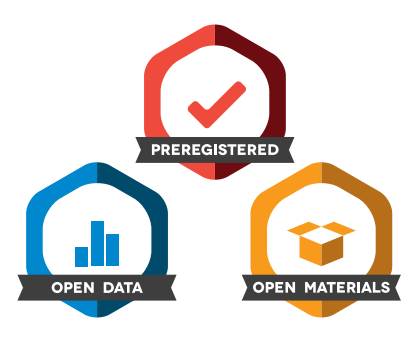
The main benefactor of publishing data and code is your future self, no one is more likely to continue your work. This should be an important incentive. Another incentive are Open Science "badges": icons presented next to the article title indicating whether the study was preregistered and provides open data and open materials (code). The introductions of these badges in the journal "Psychological Science" increased the percentage of articles with available data quickly to almost 40%.

The conference was organised by FORCE11, a community interested in future research communication and e-scholarship. There are already a lot of tools for the open, findable and well-connected world of the future, but their adoption could go faster. So the theme of this year's conference was "changing the culture".

Open Access

Christopher Jackson; on the right. (I hope I am allowed to repeat his joke.)

A main address was by Christopher Jackson. He has published over 150 scientific articles, but only became aware of how weird the scientific publishing system is when he joined ResearchGate, a social network for scientists, and was not allowed to put many of his articles on it because the publishers have the copy rights and do not allow this.

The frequent requests for copies of his articles on Research Gate also created an awareness how many scientists have trouble accessing the scientific literature due to pay-walls.

Another key note speaker, Diego Gómez, was threatened with up to eight years in jail for making scientific articles accessible. His university, Universidad del Quindio in Costa Rica, spends more on licenses for scientific journals ($375,000) than on producing scientific knowledge themselves ($253,000).



The lack of access to the scientific literature makes research in poorer countries a lot harder, but even I am regularly not able to download important articles and have to ask the authors for a copy or ask our library to order a photocopy elsewhere, although the University of Bonn is not a particularly poor university.

Also non-scientists may benefit from being able to read scientific articles, although when it is important I would prefer to consul an expert over mistakenly thinking I got the gist of an article in another field. Sometimes a copy of the original manuscript is found on one of the authors homepages or a repository. Google (Scholar) and the really handy browser add-on unpaywall can help find those using the Open Access DOI database.

Also sharing passwords and Sci-Hub are solutions, but illegal. The real solutions to making research more accessible are Open Access publishing and repositories for manuscripts. By now about half of the recently published articles are Open Access and in this pace all articles would be Open Access by 2040. Interestingly the largest fraction of the publicly available articles does not have an Open Access license, also called bronze Open Access. This means that the download possibility could also be revoked again.

The US National Institutes of Health and the European Union mandate that its supported research will be published Open Access.

A problem with Open Access journals can be that some are only interested in the publication fees and do not care about the quality. These predatory journals are bad for the reputation of real Open Access journals, especially in the eyes of the public.

I have a hard time believing that the authors do not know that these journals are predatory. Next to the sting operations to reveal that certain journals will publish anything, it would be nice to also have sting predatory journals that openly email the authors that they will accept any trash and see if that scares away the authors.

Jeffrey Beall used to keep a list of predatory journals, but had to stop after legal pressure from these frauds. The publishing firm Cabell now launched their own proprietary (pay-walled) blacklist, which already has 6000 journals and is growing fast.

Preprint repositories

Before a manuscript is submitted to a journal, the authors naturally still have the copy rights. They can thus upload the manuscript to a database, so-called preprint or institutional repositories. Unfortunately some publishers say this constitutes publishing a manuscript and they refuse to publish it because it is no longer new. However, most publishers accept the publications of the manuscript as it was before submission. A smaller part is also okay with the final version being published on the author's homepages or repositories.

Where a good option for an Open Access journal exists we should really try to use it. Where it is allowed, we should upload our manuscripts to repositories.

Good news for the readers of this blog is that a repository for the Earth Sciences was opened last week: EarthArXiv. This fall, the AGU will also demonstrate its preprint repository at the AGU Fall meeting. For details see my previous post.  EarthArXiv already has 15 climate related preprints.

This November also a new OSF ArXiv has started: MarXiv, not for Marxists, but for the marine-conservation and marine-climate sciences.

When we combine the repositories with peer review organised by the scientific community itself, we will no longer need pay-walling scientific publishers. This can be done in a much more informative way than currently where the reader only knows that the paper was apparently good enough for the journal, but not why it is a good article, not how it fits in the (later published) literature. With Grassroots scientific publishing we can do a much better job.

One way the reviews at a Grassroots journal can be better is by openly assessing the quality of the work. Now all we know is that the study was sufficiently interesting for some journal at that time for whatever reason. What I did not realise before Berlin is that this wastes a lot of time reviewing. Traditional journals waste resources on manuscripts, which are valid, but are rejected because they are seen as not important enough for the journal. For example, Frontiers reviews 2.4 million manuscripts and has to bounce about 1 million valid papers.

On average scientists pay $5,000 per published article. This while scientists do most of the work for free (writing, reviewing, editing) and while the actual costs are a few $100. The money we save can be used for research. In the light of these numbers it is actually amazing that Elsevier only makes a profit of 35 to 50%. I guess their CEO's salary eats into the profits.

Preprints would also have the advantage of making studies available faster. Open Access makes text and data mining easier, which helps in finding all articles on molecule M or receptor R. First publishers are using Text mining and artificial intelligence to suggest suitable peer reviewers to their editors. (I would prefer editors who know their field.) It would also help in detecting plagiarism and even statistical errors.

(Before our machine overlords find out, let me admit that I did not always write the model description of the weather prediction model I used from scratch.)

Impact factors

Another issue Christopher Jackson highlighted is the madness of the Journal Impact Factors (JIF or IF). They measure how often an average article in a journal is cited in the first two or five years after publication. They are quite useful for librarians to get an overview over which journals to subscribe to. The problem begins when this impact factor is used to determine the quality of a journal or the articles in it.

How common this is, is actually something I do not know. For my own field I would think I have a reasonable feeling about the quality of the journals, which is independent of the impact factor. More focussed journals tend to have smaller impact factors, but that does not signal that they are less good. Boundary Layer Meteorology is certainly not worse than the Journal of Geophysical Research. The former has in Impact Factor of 2.573, the latter of 3.454. If you made a boundary layer study it would be madness to then publish it in a more general geophysical journal where the chance is smaller that relevant colleagues will read it. Climate journals will have higher impact factors than meteorological journals because meteorologists mainly cite each other, while many sciences build on climatology. When the German meteorological journal MetZet was still a pay-wall journal it had a low impact factor because not many outside of Germany had a subscription, but the quality of the peer review and the articles was excellent.

I would hope that reviewers making funding and hiring decisions know the journals in their field and take these kind of effects into account and read the articles itself. The [[San Francisco Declaration on Research Assessment]] (DORA) rejects the use of the impact factor. In Germany it is officially forbidden to judge individual scientists and small groups based on bibliographic measures such as the number of articles times the impact factor of the journals. Although I am not sure if everybody knows this. Imperial College recently adopted similar rules:

“the College should be leading by example by signalling that it assesses research on the basis of inherent quality rather than by where it is published”
“eliminate undue reliance on the use of journal-based metrics, such as JIFs, in funding, appointment, and promotion considerations”

The relationship between the number of citations an article can expect and the impact factor is weak because there is enormous spread. Jackson showed this figure.



This could well be a feature and not a bug. We would like to measure quality, not estimate the (future) number of citations of an article. For my own articles, I do not see much correlation between my subjective quality assessment and the number of citations. Which journal you can get into may well be a better quality measure than individual citations. (The best assessment is reading articles.)

The biggest problem is when the journals, often commercial entities, start optimising for the number of citations rather than quality. There are many ways to get more citations, a higher impact factor, than making the best possible quality control. An article that reviews the state of the scientific field typically get a lot of citations, especially if writing by the main people in the field. Nearly every article will mention it in the introduction. Review papers are useful, but we do not need a new one every year. Articles with many authors typically get more citations. Articles on topics many scientists work on will get more citations. For Science and Nature it is important to get coverage in the main stream press, which is also read by scientists and leads to more citations.

Reading articles is naturally work. I would suggest to reduce the number of reviews.

Attribution, credit

Traditionally one gets credit for scientific work by being author of a scientific paper. However, with increased collaboration and interdisciplinary work author lists have become longer and longer. Also the publish or perish system likely contributed: outsourcing part of the work is often more efficient than doing it yourself, while the person doing a small part of the analysis is happy to have another paper on their publish or perish list.

What is missing from such a system is getting credit for a multitude of other import tasks. How does one value non-traditional output items supplied by researchers: code, software, data, design, standards, models, MOOC lectures, newspaper articles, blog posts, community engaged research and citizen science? Someone even mentioned musicals.

A related question is who should be credited: technicians, proposal writers, data providers? As far as I know it would be illegal to put people in such roles in author list, but they do work that is important, needs to be done and thus needs to be credited somehow. A work-around is to invite them to help in editing the manuscript, but it would be good to have systems where various roles are credited. Designing such a system is hard.

One is temped to make such a credit system very precise, but ambiguity also has its advantages to deal with the messiness of reality. I once started a study with one colleague. Most of this study did not work out and the final article was only about a part. A second colleague helped with that part. For the total work the first colleague had done more work, for the part that was published the second one. Both justifiably found that they should be second author. Do you get credit for the work or for the article?

Later the colleague who had become third author of this paper wrote another study where I helped. It was clear that I should have been the second author, but in retaliation he made me the third author. The second author wrote several emails that this was insane, not knowing what was going on, but to no avail. A too precise credit system would leave no room for such retaliation tactics to clear the air for future collaborations.

In one session various systems of credit "badges" were shown and tried out. What seemed to work best was a short description of the work done by every author, similar to a detailed credit role at the end of a movie.

This year a colleague wrote on a blog that he did not agree with a sentence of an article he was author of. I did not know that was possible; in my view authors are responsible for the entire article. Maybe we should also split up the authors list in authors who guarantee with their name and reputation for the quality of the full article and honorary authors who only contributed a small part. This colleague could then be a honorary author.

LindedIn endorsements were criticised because they are not transparent and they make it harder to change your focus because the old endorsements and contacts stick.

Pre-registration

Some fields of study have trouble replicating published results. These are mostly empirical fields where single studies — to a large part — stand on their own and are not woven together by a net of theories.

One of the problems is that only interesting findings are published and if no effect is found the study is aborted. In a field with strong theoretical expectations also finding no effect when one is expected is interesting, but if no one expected a relationship between A and B, finding no relationship between A and B is not interesting.

This becomes a problem when there is no relationship between A and B, but multiple experiments/trails are made and some will find a fluke relationship by chance. If only those get published that gives a wrong impression. This problem can be tackled by registering trails before they are made, which is becoming more common in medicine.

A related problem is p-hacking and hypothesis generation after results are known (HARKing). A relationship which is statistically significant if only one outlier were not there, makes it tempting to find a reason why the outlier is a measurement error and should be removed.

Similarly the data can be analyses in many different ways to study the same question, one of which may be statistically significant by chance. This is also called "researcher degrees of freedom" or "the garden of forking paths". The Center for Open Science has made a tool where you can pre-register your analysis before the data is gathered/analysed to reduce the freedom to falsely obtain significant results this way.



A beautiful example of the different answers one can get analysing the same data for the same question. If found this graph via a FiveThirtyEight article, which is also otherwise highly recommended: "Science Isn’t Broken. It’s just a hell of a lot harder than we give it credit for."

These kind of problems may be less severe in natural sciences, but avoiding them can still make the science more solid. Before Berlin I was hesitant about pre-registering the analysis because in my work every analysis is different, which makes is harder to know in detail in advance how the analysis should go; there are also valid outlier that need to be removed, selecting the best study region needs a look at the data, etc.

However, what I did not realise, although quite trivial, is that you can do the pre-registered analysis, but also additional analysis and simply mark them as such. So if you can do a better analysis after looking at the data, you can still do so. One of the problems of pre-registering is that quite often people did not do the analysis in the same way and that reviewers mostly do not check this.

In the homogenisation benchmarking study of the ISTI we will describe the assessment measures in advance. This is mostly because the benchmarking participants have a right to know how their homogenisation algorithms will be judged, but it can also be seen as pre-registration of the analysis.

To stimulate the adoption of pre-registration, the Center for Open Science has designed Open Science badges, which can be displayed with the articles meeting the criteria. The pre-registration has to be done at an external site where the text cannot be changed afterwards. The pre-registration can be kept undisclosed for up to two years. To get things started they even award 1000 prices of $1000 for pre-registered studies.

The next step would be journals that review "registered reports", which are peer reviewed before the results are in. This should stimulate the publication of negative (no effect found) results. (There is still a final review when the results are in.)

Quick hits

Those were the main things I learned, now some quick hits.

With the [[annotation system]] you can add comments to all web pages and PDF files. People may know annotation from Hypothes.is, which is used by ClimateFeedback to add comments to press articles on climate change. A similar initiative is PaperHive. PaperHive sells its system as collaborative reading and showed an example of students jointly reading a paper for class, annotating difficult terms/passages. It additionally provides channels for private collaboration, literature management and search. It has also already been used for the peer review (proof reading) of academic books. They now both have groups/channels to allow groups to make or read annotations, as well as private annotations, which can be used for your own paper archive. Web annotations aimed at the humanities are made by Pund.it.

Since February this year, web annotation is a World Wide Web (W3C) standard. This will hopefully mean that web browsers will start adding annotation in their default configuration and it will be possible to comment every homepage. This will likely lead to public annotation streams going down to the level of YouTube comments. Also for the public channel some moderation will be needed, for example to combat doxing. PaperHive is a German organisation and thus removes hate speech.

Peer Community In (PCI) a system to collaboratively peer review manuscripts that can later be send to an official journal.

The project OpenUp studied a large number of Open Peer Review systems and their pros and cons.

Do It Yourself Science. Not sure it is science, but great when people are having fun with science. When the quality level is right, you could say it is citizen science led by the citizens themselves. (What happened to the gentlemen scientists?)

Philica: Instant academic publishing with transparent peer-review.

"Standards are like toothbrushes; everyone likes the idea of them, but everyone wants to use their own" #FORCE2017 @Metadata2020

— Juan Pablo Alperin (@juancommander) 26 October 2017

Unlocking references from the literature: The Initiative for Open Citations. See also their conference abstract.

I never realised there was an organisation behind the Digital Object Identifiers for scientific articles: CrossRef. It is a collaboration of about eight thousand scientific publishers. For other digital sources there are other organisation, while the main system is run by the international DOI Foundation. The DOIs for data are handled, amongst others, by DataCite. CrossRef is working on a system where you can also see the webpages that are citing scientific articles, what they call "event data". For example, this blog has cited 142 articles with a DOI. CrossRef will also take web annotations into account.

Climate science was well represented at this conference. There were posters on open data for the Southern Ocean and on the data citation of the CMIP6 climate model ensemble. Shelley Stall of AGU talked about making FAIR and Open data the default for Earth and space science. (Et moi.)



In the Life Sciences they are trying to establish "micro publications", the publication of a small result or dataset, several of which can then later be combined with a narrative into a full article.

A new Open Science Journal: Research Ideas and Outcomes (RIO), which publishes all outputs along the research cycle, from research ideas, proposals, to data, software and articles. They are interested in all areas of science, technology, humanities and the social sciences.

Collaborative writing tools are coming of age, for example, Overleaf for people using LaTex. Google Docs and Microsoft Word Live also do the trick.

Ironically Elsevier was one of the sponsors. Their brochure suggests they are ones of the nice guys serving humanity with cutting edge technology.

The Web of Knowledge/Science (a more selective version of Google Scholar) moved from Thomson Reuters to Clarivate Analytics, together with the Journal Citation Reports that computes the Journal Impact Factors.

Publons has set up a system where researchers can get public credit for their (anonymous) peer reviews. It is hoped that this stimulates scientists to do more reviews.

As part of Wikimedia, best known for Wikipedia, people are building up a multilingual database with facts: wikidata. Like in Wikipedia volunteers build up the database and sources need to be cited to make sure the facts are right. People are still working on software to make contributing easier for people who are not data scientists and do not dream of the semantic web every night.

Final thoughts

For a conference about science, there was relatively little science. One could have made a randomized controlled trial to see the influence of publishing your manuscript on a preprint server. Instead the estimated larger number of citations for articles also submitted to ArXiv (18%) was based on observational data and the difference could be that scientists put more work in spreading their best articles.

The data manager at CERN argued that close collaboration with the scientists can help in designing interfaces that promote the use of Open Science tools. Sometimes small changes produce large increases in adoption of tools. More research into the needs of scientists could also help in creating the tools in a way that they are useful.

Related reading, resources

The easiest access to the talks of the FORCE2017 conference is via the "collaborative note taking" Google Doc

Videos of last year's FORCE conference

Peer review

The Times Literary Supplement: Peer review: The end of an error? by ArXiving mathematician Timothy Gowers

Peer review at the crossroads: overview over the various open review options, advantages and acceptance

Jon Tennant and many colleagues: A multi-disciplinary perspective on emergent and future innovations in peer review

My new idea: Grassroots scientific publishing

Pre-prints

The Earth sciences no longer need the publishers for publishing
 
ArXivist. A Machine Learning app that suggest the most relevant new ArXiv manuscripts in a daily email

The Stars Are Aligning for Preprints. 2017 may be considered the ‘year of the preprint

Open Science

The State of OA: A large-scale analysis of the prevalence and impact of Open Access articles

Open Science MOOC (under development) already has an extensive resources page

Metadata2020: Help us improve the quality of metadata for research. They are interested in metadata important for discoverability and reuse of data

‘Kudos’ promises to help scientists promote their papers to new audiences. For example with plain-language summaries and tools measure which dissemination actions were effective

John P. A. Ioannidis and colleagues: Bibliometrics: Is your most cited work your best? Survey finds that highly cited authors feel their best work is among their most cited articles. It is the same for me, still looking at all articles it is not a strong correlation

Lorraine Hwang and colleagues in Earth and Space Science: Software and the scientist: Coding and citation practices in geodynamics, 2017

Neuroskeptic: Is Reproducibility Really Central to Science?

With some programing skills you can compute global mean temperatures yourself

This is a guest post by citizen scientist Ron Roeland (not his real name, but I like alliteration for some reason). Being an actually sceptical person, he decided to compute the global mean land temperature from station observations himself. He could reproduce the results of the main scientific groups that compute this signal and, new for me, while studying the data noticed how important the relocation of temperature stations to airports is for the NOAA GHCNv3 dataset. (The headers in the post are mine.)

This post does not pretend to present a rigorous analysis of the global temperature record; instead, it intends to show how easy it is for someone with basic programming/math skills to debunk claims that NASA and NOAA have manipulated temperature data to produce their global-average temperature results, i.e. claims like these:

From C3 Headlines: By utilizing questionable adjustments based on even more questionable assumptions, NOAA managed to produce an entirely fabricated increase in the global warming trend from 1998 to 2012.

From a blogger on the Hill: There’s going to have to be a massive effort to pick apart failing climate models and questionably-adjusted data.

From Climate Depot: Over the past decade, NASA and NOAA have continuously altered the temperature record to cool the past and warm the present. Their claims are straight out Orwell's 1984, and have nothing to do with science'

The routine

Some time ago, after reading all kinds of claims (like the ones above) about how NASA and NOAA had improperly adjusted temperature data to produce their global-average temperature results, I decided to take a crack at the data myself.

I coded up a straightforward baselining/gridding/averaging routine that is quite simple and “dumbed down” in comparison to the NASA and NOAA algorithms. Below is a complete description of the algorithm I coded up.

1. Using GHCN v3 monthly-average data, compute 1951-1980 monthly baseline temperatures for all GHCN stations. If a station has 15 or more valid temperatures in any given month for the 1951-1980 baseline period, retain that monthly baseline value; otherwise drop that station/month from the computations. Stations with no valid monthly baseline periods are completely excluded from the computations.
2. For all stations and months where valid baseline temperature estimates were computed per (1) above, subtract the respective baseline temperatures from all of the station monthly temperature temperatures to produce monthly temperature anomalies for the years 1880-2015.
3. Set up a global gridding scheme to perform area-weighting. To keep things really simple, and to minimize the number of empty grid-cells, I selected large grid-cell sizes (20 degrees x 20 degrees at the Equator). I also opted to recalculate the grid-cell latitude dimensions as one goes north/south of the equator in order to keep the grid-cell areas as nearly constant as possible. I did this to keep the grid-cell areas from shrinking (per the latitude cosines) in order to minimize the number of empty grid cells.
4. In each grid-cell, compute the average (over all stations in the grid-cell) of the monthly temperature anomalies to produce a single time-series of average temperature anomalies for each month (years 1880 through 2015).
5. Compute global average monthly temperature anomalies by averaging together all the grid-cell monthly average anomalies, weighted by the grid-cell areas (again, for years 1880 through 2015).
6. Compute global-average annual anomalies for years 1880 through 2015 by averaging together the global monthly anomalies for each year.

The algorithm does not involve any station data adjustments (obviously!) or temperature interpolation operations. It’s a pretty basic number-crunching procedure that uses straightforward math plus a wee bit of trigonometry (for computing latitude/longitude grid-cell areas).

For me, the most complicated part of the algorithm implementation was managing the variable data record lengths and data gaps (monthly and annual) in the station data -- basically, the “data housekeeping” stuff. Fortunately, modern development libraries such as the C++ Standard Template Library make this less of a chore than it used to be.

Why this routine?

People unfamiliar with global temperature computational methods sometimes ask: “Why not simply average the temperature station data to compute global-average estimates? Why bother with the baselining and gridding described above?”

We could get away with straight averaging of the temperature data if it were not for the two problems described below.

Problem 1: Temperature stations have varying record lengths. The majority of stations do not have continuous data records that go all the way back to 1880 (the beginning of the NASA/GISS global temperature calculations). Even stations with data going back to 1880 have gaps in their records -- there are missing months or even years.

Problem 2: Temperature stations are not evenly distributed over the Earth’s surface. Some regions, like the continental USA and western Europe, have very dense networks of stations. Other regions, like the African continent, have very sparse station networks.

As a result of problem 1, we have a mix of temperature stations that changes from year to year. If we were simply to average the absolute temperature data from all those stations, the final global-average results would be significantly skewed from year to year due to the changing mix of stations from one year to the next.

Fortunately, the solution for this complication is quite straightforward: the baselining and anomaly-averaging procedure described above. For those who already familiar with this procedure, please bear with me while I illustrate how it works with a simple scenario constructed from simulated data.

Let’s consider a very simple scenario where the full 1880-2016 temperature history for a particular region is contained in data reported by two temperature stations, one of which is located on a hilltop and the other located on a nearby valley floor. The hilltop and valley floor locations have identical long-term temperature trends, but the hilltop location is consistently about 1 degree C cooler than the valley floor location. The hilltop temperature station has a temperature record starting in 1880 and ending in 1990. The valley floor station has a temperature record beginning in 1930 and ending in 2016.

Figure 1 below shows the simulated temperature time-series for these two hypothetical stations. Both time-series were constructed by superimposing random noise on the same linear trend, with the valley-floor station time-series having a constant offset temperature 1 degree C more than that of the hilltop station time-series. The simulated time-series for the hilltop station (red) begins in 1880 and continues to 1990. The simulated valley floor station temperature (blue) data begins in 1930 and runs to 2016. As can be seen during their period of overlap (1930-1990), the simulated valley-floor temperature data runs about 1 degree warmer than the simulated hilltop temperature data.


Figure 1: Simulated Hilltop Station Data (red) and Valley Floor Station Data (blue)

If we were to attempt to construct a complete 1880-2016 temperature history for this region by computing a straight average of the hilltop and valley floor data, we would obtain the results seen in Figure 2 below.


Figure 2: Straight Average of Valley Floor Station Data and Hilltop Station Data

The effects of the changing mix of stations (hilltop vs. valley floor) on the average temperature results can clearly be seen in Figure 2. A large temperature jump is seen at 1930, where the warmer valley floor data begins, and a second temperature jump is seen at 1990 where the cooler hilltop data ends. These temperature jumps obviously do not represent actual temperature increases for that particular region; instead, they are artifacts introduced by the changes in the mix of stations in 1930 and 1990.

An accurate reconstruction of the regional temperature history computed from these two temperature time-series obviously should show the warming trend seen in the hilltop and valley floor data over the entire 1880-2016 time period. That is clearly not the case here. Much of the apparent warming seen in Figure 2 is a consequence of the changing mix of stations.

Now, let’s modify the processing a bit by subtracting the (standard NASA/GISS) 1951-1980 hilltop baseline average temperature from the hilltop temperature data and the 1951-1980 valley floor baseline average temperature from the valley floor temperature data. This procedure produces the temperature anomalies for the hilltop and valley floor stations. Then for each year, compute the average of the station anomalies for the 1880-2016 time period.

This is the baselining and anomaly-averaging procedure that is used by NASA/GISS, NOAA, and other organizations to produce their global-average temperature results.

When this baselining and anomaly-averaging procedure is applied to the simulated temperature station data, it produces the results that can be viewed in figure 3 below.


Figure 3: Average of Valley Floor Station Anomalies and Hilltop Station Anomalies

In Figure 3, the temperature jumps associated with the beginning of the valley floor data record and the end of the hilltop data record have been removed, clearly revealing the underlying temperature trend shared by the two temperature time-series.

Also note that although neither of my simulated temperature stations have a full 1880-2016 temperature record, we were still able to compute a complete reconstruction for the 1880-2016 time period because there was enough overlap between the station records to allow us to “align” them via baselining.

The second problem, the non-uniform distribution of temperature stations, can clearly be seen in Figure 4 below. That figure shows all GHCNv3 temperature stations that have data records beginning in 1900 or earlier and continuing to the present time.


Figure 4: Long-Record GHCN Station Distribution

As one can see, the stations are highly concentrated in the continental USA and western Europe; Africa and South America, in contrast, have very sparse coverage. A straight unweighted average of the data from all the stations shown in the above image would result in temperature changes in the continental USA and western Europe “swamping out” temperature changes in South America and Africa in the final global average calculations.

That is the problem that gridding solves. The averaging procedure using grid-cells is performed in two steps. First, the temperature time-series for all stations in each grid-cell are averaged together to produce a single time-series per grid-cell. Then all the grid-cell time-series are averaged together to construct the final global-average temperature results (note: in the final average, the grid-cell time-series are weighted according to the size of each grid-cell). This eliminates the problem where areas on the Earth with very dense networks of stations are over-weighted in the global average relative to areas where the station coverage is more sparse.

Now, some have argued that the sparse coverage of certain regions of the Earth invalidate the global-average temperature computations. But it turns out that the NASA/GISS warming trend can be confirmed even with a very sparse sampling of the Earth’s surface temperatures. (In fact, the NASA/GISS warming trend can be replicated very closely with data from as few as 30 temperature stations scattered around the world.)

Real-world results

Now that we are done with the preliminaries, let’s look at some real-world results. Let’s start off by taking a look at how my simple “dumbed-down” gridding/averaging algorithm compares with the NASA/GISS algorithm when it is used to process the same GHCNv3 adjusted data that NASA/GISS uses. To see how my algorithm compares with the NASA/GISS algorithm, take a look at Figure 5 below, where the output of my algorithm is plotted directly against the NASA/GISS “Global Mean Estimates based on Land Data only” results.

(Note: All references to NASA/GISS global temperature results in this post refer specifically to the NASA/GISS “Global Mean Estimates based on Land Data only” results. Those results can be viewed on the NASA/GISS web-site; scroll down to view the “Global Mean Estimates based on Land Data only” graph).


Figure 5: Adjusted Data, All Stations: My Simple Gridding/Averaging (blue) vs. NASA/GISS (red)

In spite of the rudimentary nature of my algorithm, my algorithm produces results that match the NASA/GISS results quite closely. According to the R-squared statistic I calculated (seen in the upper-left corner of Figure 5), I got 98% of the NASA/GISS answer with a only tiny fraction of the effort!

But what happens when we use unadjusted GHCNv3 data? Well, let’s go ahead and compare the output of my algorithm with the NASA/GISS algorithm when my algorithm is used to process the unadjusted GHCNv3 data. Figure 6 below shows a plot of my unadjusted global temperature results vs. the NASA/GISS results (remember that NASA/GISS uses adjusted GHCNv3 data).


Figure 6: Unadjusted Data, All Stations: My Simple Gridding /Averaging (green) vs. NASA/GISS (red)

My “all stations” unadjusted data results show a warming trend that lines up very closely with the NASA/GISS warming trend from 1960 to 2016, with my results as well as the NASA/GISS results showing record high temperatures for 2016. However, my results do show a visible warm-bias relative to the NASA/GISS results prior to 1950 or so. This is the basis of the accusations that NOAA and NASA “cooled the past (and warmed the present)” to exaggerate the global warming trend.

Now, why do my unadjusted data results show that pre-1950 “warm bias” relative to the NASA/GISS results? Well, this excerpt from NOAA’s GHCN FAQ provides some clues:

Why are there more cold (negative) step changes than warm(positive) step changes in the historical land surface air temperature records represented in the GHCN v3 dataset?

The reason for the larger number of cold step changes is not completely clear, but they may be due in part to systematic changes in station locations from city centers to cooler airport locations that occurred in many parts of the world from the 1930s to through the 1960s.

Because the GHCNv3 metadata contains an airport designator field for every temperature station, it was quite easy for me to modify my program to exclude all the “airport” stations from the computations. So let’s exclude all of the “airport” station data and see what we get. Figure 7 below shows my unadjusted data results vs. the NASA/GISS results when all “airport” stations are excluded from my computations.


Figure 7: Unadjusted Data, Airports Excluded (green) vs. NASA/GISS (red)

There is a very visible reduction in the bias between my unadjusted results and the NASA results (especially prior to 1950 or so) when airport stations are excluded from my unadjusted data processing. This is quite consistent with the notion that many of the stations currently located at airports were moved to their current locations from city centers at some point during their history.

Now just for fun, let’s look at what happens when we do the reverse and exclude non-airport stations (i.e. process only the airport stations). Figure 8 shows what we get when we process unadjusted data exclusively from “airport” stations.


Figure 8: Unadjusted Data, Airports Only (green) vs. NASA/GISS (red)

Well, look at that! The pre-1950 bias between my unadjusted data results and the NASA/GISS results really jumps out. And take note of another interesting thing about the plot -- in spite of the fact that I processed only “airport” stations, the green “airports only” temperature curve goes all the way back to 1880, decades prior to the existence of airplanes (or airports)! It is only reasonable to conclude that those “airport” stations must have been moved at some point in their history.

Now, for a bit more fun, let’s drill down a little further into the data and process only airport stations that also have temperature data records going back to 1903 (the year that the Wright Brothers first successfully flew an airplane) or earlier.

When I drilled down into the data, I found over 400 “airport” temperature stations with data going back to 1903 or earlier. And when I computed global-average temperature estimates from just those stations, this is what I got (Figure 9):


Figure 9: Unadjusted Data, Airport Stations with pre-1903 Data (green) vs. NASA/GISS (red)

OK, that looks pretty much like the previous temperature plot, except that my results are “noisier” due to the fact that I processed data from fewer temperature stations.

And for even more fun, let’s look at the results we get when we process data exclusively from non-airport stations with data going back to 1903 or earlier:


Figure 10: Unadjusted Data, Non-Airport Stations with pre-1903 Data (green) vs. NASA/GISS (red)

When only non-airport stations are processed, the pre-1950 “eyeball estimate” bias between my unadjusted data temperature curve and the NASA/GISS temperature curve is sharply reduced.

The results seen in the above plots are entirely consistent with the notion that the movement of large numbers of temperature stations from city centers to cooler outlying airport locations during the middle of the 20th Century is responsible for much of the bias seen between the unadjusted and adjusted GHCNv3 global-average temperature results.

It is quite reasonable to conclude, based on the results presented here, that one major reason for the bias seen between the GHCNv3 unadjusted and adjusted data results is the presence of corrections for those station moves in the adjusted data (corrections that are obviously absent from the unadjusted data). Those corrections remove the contaminating effects of station moves and permit more accurate estimates of global surface temperature increases over time.

Take-home lessons (in no particular order):

1. Even a very simple global temperature algorithm can reproduce the NASA/GISS results very closely. This really is a case where you can get 98% of the answer (per my R-squared statistic) with less than 1% of the effort.
2. NOAA’s GHCNv3 monthly data repository contains everything an independent “citizen scientist” needs (data and documentation) to conduct his/her own investigation of the global land station temperature data.
3. A direct comparison of unadjusted data results (all GHCN stations) vs. the NASA/GISS adjusted data temperature curves reveals only modest differences between the two temperature curves, especially for the past 6 decades. Furthermore, my unadjusted and the NASA/GISS adjusted results show nearly identical (and record) temperatures for 2016. If NASA and NOAA were adjusting data to exaggerate the amount of planetary warming, they sure went to an awful lot of trouble and effort to produce only a small overall increase in warming in the land station data.
4. Eliminating all “airport” stations from the processing significantly reduced the bias between my unadjusted data results and the NASA/GISS results. It is therefore reasonable to conclude that a large share of the modest bias between my GHCN v3 unadjusted results and the NASA/GISS adjusted data results is the result of corrections for station moves from urban centers to outlying airports (corrections present in the adjusted data, but not in the unadjusted data).
5. Simply excluding “airport” stations likely eliminates many stations that were always located at airports (and never moved) and also fails to eliminate stations that were moved out from city centers to non-airport locations. So it is not a comprehensive evaluation of the impacts of station moves. However, it is a very easy “first step” analysis exercise to perform; even this incomplete “first step” analysis produces results that strongly consistent with the hypothesis that corrections for station moves are likely the dominant reason for the pre-1950 bias seen between the adjusted and unadjusted GHCN global temperature results. Remember that many urban stations were also moved from city centers to non-airport locations during the mid-20th century. Unfortunately, those station moves are not recorded in the simple summary metadata files supplied with the GHCNv3 monthly data. An analysis of NOAA’s more detailed metadata would be required to identify those stations and perform a more complete analysis of the impacts of station moves. However, that is outside of the scope of this simple project.
6. For someone who has the requisite math and programming skills, confirming the results presented here should not be very hard at all. Skeptics should try it some time. Provided that those skeptics are willing and able to accept results that contradict their original views about temperature data adjustments, they could have a lot of fun taking on a project like this.

Related reading

Also the Clear Climate Code project was able to reproduce the results of NASA-GISS. Berkeley Earth made an high-level independent analysis and confirmed previous results. Also (non-climate) scientist Nick Stokes (Moyhu) computed his own temperature signal: TempLS which also fits well.

In 2010 Zeke Hausfather analyzed the differences in GHCNv2 between airport and other stations and found only minimal differences: Airports and the land temperature record.

At about the same time David Jones at Clear Climate Code also looked at airport station, just splitting the dataset in two groups, and did found differences: Airport Warming. Thus making sure both groups are regionally comparable is probably important.

The global warming conspiracy would be huge. Not only the 7 global datasets also national datasets from so many groups show clear warming.

Just the facts, homogenization adjustments reduce global warming.

Why raw temperatures show too little global warming.

Irrigation and paint as reasons for a cooling bias.

Temperature trend biases due to urbanization and siting quality changes.

Temperature bias from the village heat island

Cooling moves of urban stations. From cities to airports or simply to outside a city or village.

The transition to automatic weather stations. We’d better study it now. It may be a cooling bias.

Changes in screen design leading to temperature trend biases.

Early global warming

Cranberry picking short-term temperature trends

How climatology treats sceptics

Extending the temperature record of southeastern Australia

This is a guest post by Linden Ashcroft. She did her PhD studying non-climatic changes in the early instrumental period in Australia and now works at the homogenization power house, the Centre on Climate Change (C3) in Tarragona, Spain. She weekly blogs on homogenization and life in Spain.

This guest post was originally written for the Climanrecon blog. Climanrecon is currently looking at the non-climatic features of the Bureau of Meteorology’s raw historical temperature observations, which are freely available online. As Neville Nicholls recently discussed in The Conversation, the more the merrier!

---

Southeastern Australia is the most highly populated and agriculturally rich area in Australia. It’s home to our tallest trees, our highest mountains, our oldest pubs and most importantly, our longest series of instrumental weather observations. This makes southeastern Australia the most likely place to extend Australia’s instrumental climate record.

The official Australian Bureau of Meteorology was formed in 1908, bringing standard observing practices into effect across the country. Before this time, Australian weather station coverage was not as dense as today’s network, and there was no nationally-standard procedure for recording temperature.

The uncertain quality of the pre-1910 data and the lack of readily available information about observation techniques is why the current high-quality temperature dataset available for Australia does not begin until 1910. However, this does not mean that valuable observations were not taken in the 19th century, or that the spatial coverage of these data is too poor to be useful for studies of regional climate. Here, I explain what colleagues and I did to extend the temperature record of southeastern Australia.

When is the temperature not the temperature?

First of all, it’s important to know what ‘non-climatic’ influences can affect temperature observations. Some influences are fairly obvious: if you move a thermometer 20km down the road, change the time of day that the temperature is recorded, or replace the screen the thermometer is housed in, that will most likely cause changes in the data recorded at that station which are not caused by actual changes in the surrounding air.

Other non-climatic influences are more subtle. The slow growth of a tree next to a thermometer for example, or changes to the irrigation system in nearby paddocks can cause gradual changes to temperature observations that are not a reflection of the temperature in the wider area.

Three thermometer screens used in Adelaide, South Australia, in 1890: a Stevenson screen (left), a thermometer shed (centre), and a Glaisher stand (right). Charles Todd famously recorded the temperature in each of these screens for around 40 years, giving us invaluable information about the effect of different screens on temperature observations. Image: Meteorological Observations Made at the Adelaide Observatory, Charles Todd (1907).

Finding and reducing the impacts of these non-climatic influences is an important part of any climate change research. A multitude of statistical methods have been developed over the last 30 or so years to do this, ranging from the beautifully simple to the mind-bogglingly complex. Most of these methods rely on reference series, or a version of the truth with which you can compare data from the station you’re interested in. Reference series are often made using data from neighbouring weather stations that experience a similar climate. Of course this is much harder if you don’t have many neighbouring stations, or if a change in observation method happens at all stations at once! This is another reason why Australia’s national temperature record does not extend before 1910.

As well as these statistical tests, it’s also really useful to have information, or metadata, about the maintenance and changes that occur at a weather station. Metadata help you understand why a non-climatic influence might occur in the climate data, and how big it could be. In reality though, metadata can be hard to find.

Extending southeastern Australia’s temperature record

My work with the South Eastern Australian Recent Climate History project (SEARCH) set out to explore the quality and availability of climate data for Australia before 1908. Our aim was not to look at extreme events, or the exact temperature value at a particular location in a particular month, but to see how the average temperature across southeastern Australia varied over years and decades. This is important to note because if we were studying extremely hot months for example, or only the climate of Wagga, we might have used different methods.

The first step was looking for long-term temperature stations in southeastern Australia. Although the Bureau of Meteorology only started in 1908, a number of weather stations were set up in capital cities and key country towns from the late 1850s, thanks to the dedication of Australia’s Government Astronomers and Meteorologists

My colleagues and I also uncovered some sources of pre-1860 instrumental climate data for southeastern Australia that we painstakingly digitised and prepared for analysis. You can read more about that here.

Next, we spent a lot of time collecting information from the Bureau of Meteorology and previous studies about possible changes in station locations and other things that might affect the quality of the observational data. For some stations we found a lot of photos and details about changes to the area around a weather station. For others, particularly in the pre-1860 period, we didn’t find much at all.

After getting all this information and removing some outlying months, we tried to identify the non-climatic features of the temperature observations, and remove their influence. For the pre-1860 data this was particularly difficult, because we did not have a lot of metadata and there were no nearby stations to use as a ‘truth’. In the end we looked for large changes in the data that were supported by metadata and by the behaviour of other variables.

For example, a drop in temperature in the 1840s at some stations occurred at the same time as an increase in rainfall, suggesting that the temperature change was real, not due to some non-climatic influence. We also noted any other issues with the data, such as a bias towards rounding temperature values to the nearest even number (a common issue in early observations).

For the post-1860 data, we applied a 2-stage process of removing the non-climatic factors, using the statistical RHtest developed by members of the international Expert Team on Climate Change Detection and Indices (ETCCDI). The first stage looked for absolute non-climatic features: big jumps in the data that were clearly instrument problems or station changes, and that were supported by the metadata.

The second stage used reference series made from the average of data from up to five highly correlated neighbouring stations. Both stages involved carefully comparing the statistical results with the metadata we had, and making a decision on whether or not a non-climatic feature was present. You can read more about the methods here.

An example of the non-climatic features, or jumps, found in Newcastle maximum temperature data from 1860–1950 using the RHtest method. The supporting metadata are also shown. Image supplied by author.

So what did we find?

Our results for the 1860–1950 period found 185 non-climatic features in the maximum temperature data, and 190 in the minimum temperature data over the full network of 38 stations. Over 50% of these non-climatic features identified were supported by metadata, and most of them occurred from 1880 to 1900, when the thermometer shelters that were used in Australia were changed from Glaisher stands to Stevenson screens.

You can see in the figures below that removing the non-climatic features had a big impact on the variance of the observations, making the spread of temperatures across the region much more similar to the post-1910 period, when observations are more reliable. Our results also agreed very well with southeastern Australia data from the Bureau of Meteorology’s monthly and daily temperature datasets that have been tested for non-climatic features using different methods.

This good agreement allowed us to combine the area-average of my data with that of the Bureau’s best temperature dataset (ACORN-SAT), building a monthly temperature record for southeastern Australia from 1860 to the present. Combining the two series showed that the current warming trends in Australia are the strongest and most significant since at least 1860.

Area-averaged SEA annual anomalies (°C, relative to the 1910–1950 base period) of original data from the historical sources (1860–1950, dashed line), adjusted data from historical sources (1860–1950, solid red line) and data from ACORN-SAT, the Bureau of Meteorology’s daily temperature data over SEA (1910–1950, solid blue line) for maximum and minimum temperature over 1860–1950. The maximum and minimum anomalies for each year across the network are also plotted for the original historical data (grey shading with black outline), adjusted historical data (pink shading with red outline) and ACORN-SAT data (blue dotted lines). Adapted from Ashcroft et al. 2012.

The 1788–1860 data had some non-climatic influences as well, but these were much harder to untangle from the true climate signal because there is not as much ‘truth’ to compare to. We identified five clear non-climatic features of the pre-1860 temperature data from three stations, and found that the year-to-year temperature changes of the adjusted data matched up pretty well with rainfall observations, and newspaper reports at the time. The quality and distribution of the pre-1860 data made it impossible to accurately combine the pre- and post-1860 observations, but hopefully in the future we will uncover more observations and can look more closely at the 1788–1860 period.

Our work is one of the first projects to tackle Australia’s pre-1910 temperature data, shedding more light on Australia’s climatic past. This research also makes use of the hard work that was done by some of the country’s scientific pioneers, which is very rewarding to me as a scientist.

But science is always moving forwards, and our work is just one link in the chain. As more statistical methods are developed and additional data uncovered, I’m sure that we, professional and citizen scientists alike, will be able to build on this work in the future.

More information and references:

Ashcroft, L., Gergis, J. and Karoly, D.J., 2014. A historical climate dataset for southeastern Australia. Geosciences Data Journal, 1(2): 158–178, DOI: 10.1002/gdj3.19 (html and PDF). You can also access the 1788–1860 data at https://zenodo.org/record/7598.

Ashcroft, L., Karoly, D.J. and Gergis, J., 2012. Temperature variations of southeastern Australia, 1860–2011. Australian Meteorological and Oceanographic Journal 62: 227–245. Download here (PDF).