Wednesday, September 30, 2015

UK global warming policy foundation (GWPF) not interested in my slanted questions

Mitigation sceptics like to complain that climate scientists do not want to debate them, but actually I do not get many informed questions about station data quality at my blog and when I come to them my comments are regularly snipped. Watts Up With That (WUWT) is a prominent blog of the mitigation sceptical movement in the US and the hobby of its host, Anthony Watts, is the quality of station measurements. He even set up a project to make pictures of weather stations. One might expect him to be thrilled to talk to me, but Watts hardly ever answers. In fact last year he tweeted: "To be honest, I forgot Victor Venema even existed." I already had the impression that Watts does not read science blogs that often, not even about this own main topic.

Two years ago Matt Ridley, adviser to the Global Warming Policy Foundation (GWPF), published an erroneous post on WUWT about the work of two Greek colleagues, Steirou and Koutsoyiannis. I had already explained the errors in a three year old blog post and thus wanted to point the WUWT readers to this mistake in a polite comment. This comment got snipped and replaced with:
[sorry, but we aren't interested in your slanted opinion - mod]
Interesting. I think such a response tells you a lot about a political movement and whether they believe themselves that they are a scientific movement.

Now the same happened on the homepage of the Global Warming Policy Foundation (GWPF).

To make accurate estimates of how much the climate has changed, scientists need to remove other changes from the observations. For example, a century ago thermometers were not protected as well against (solar) radiation as they are nowadays and the observed land station temperatures were thus a little too high. In the same period the sea surface temperature was measured by taking a bucket of water out of the sea. While the measurement was going on, the water cooled by evaporation and the measured temperature was a little too low. Removing such changes makes the land temperature trend 0.2°C per century stronger in the NOAA dataset, while removing such changes from the sea surface temperature makes this trend smaller by about the same amount. Because the oceans are larger, the global mean trend is thus made smaller by climatologists.

Selecting two regions where upward land surface temperature adjustments were relatively large, Christopher Booker accused scientists of fiddling with the data. In these two Telegraph articles he naturally did not explain his readers how large the effect is globally, nor why it is necessary, nor how this is done. That would have made his conspiracy theory less convincing.

That was the start for the review of the Global Warming Policy Foundation (GWPF). Christopher Booker wrote:
Paul [Homewood], I thought you were far too self-effacing in your post on the launching of this high-powered GWPF inquiry into surface temperature adjustments, It was entirely prompted by the two articles I wrote in the Sunday Telegraph on 24n January and 7 February, which as I made clear at the time were directly inspired by your own spectacular work on South America and the Arctic.
Not a good birth and Stoat is less impressed by the higher powers of the GWPF.

This failed birth resulted in a troubled childhood by giving the review team a list of silly loaded questions.

This troubled childhood was followed by an adolescence in disarray. The Policy Foundation asked everyone to send them responses to the silly loaded questions. I have no idea why. A review team should know the scientific literature themselves. It is a good custom to ask colleagues for advice on the manuscript, but a review team normally has the expertise to write a first draft themselves.

I was surprised that there were people willing to submit something to this organization. Stoat found two submissions. If Earth First! would make a review on the environmental impact of coal power plants, I would also not expect many submissions from respected sources.

When you ask people to help you and they invest their precious life time into writing responses for you, the least you can do is read the submissions carefully, give them your time, publish them and give a serious response. The Policy Foundation promised: "After review by the panel, all submissions will be published and can be examined and commented upon by anyone who is interested."

Nick Stokes submitted a report in June and recently found out the the Policy Foundation had wimped out and had changed their plans in July:
"The team has decided that its principal output will be peer-reviewed papers rather than a report.
Further announcements will follow in due course."
To which Stokes replied on his blog:
"So...no report! So what happens to the terms of reference? The submissions? How do they interact with "peer-reviewed papers"?"
The review team of the Policy Foundation now walked back. Its chairman, Terence Kealey a British biochemist, wrote this Tuesday:
"The panel has decided that its primary output should be in the form of peer-reviewed papers rather than a non-peer reviewed report. Work is ongoing on a number of subprojects, each of which the panel hopes will result in a peer reviewed paper.
One of our projects is an analysis of the numerous submissions made to the panel by members of the public. We anticipate that the submissions themselves will be published as an appendix to that analysis when it is published."
That sounded good. The review panel focussing on doing something useful, rather than answering their ordained silly loaded questions. And they would still take the submission somewhat seriously. Right? The text is a bit vague so I asked in the comments:
"How many are "numerous submissions"?
Any timeline for when these submissions will be published?"
I thought that was reasonably politely formulated. But these questions were removed within minutes. Nick Stokes happened to have see them. Expecting this kind of behaviour by now, after a few years in this childish climate "debate", I naturally made the screen shot below.

Interesting. I think such a response tells you a lot about a political movement and whether they believe themselves that they are a scientific movement.

[UPDATE. Reminder to self: next time look in spam folder before publishing a blog post.

Yesterday evening, I got a friendly mail by the administrator of the GWPF review homepage, Andrew Montford, better known to most as the administrator of the UK mitigation sceptical blog Bishop Hill. A blog where people think it is hilarious to remove the V from my last name.

He wrote that the GWPF newspage was not supposed to have comments, that my comment was therefore (?) removed. Montford was also so kind to answer my questions:
1. Thirty-five.
2. This depends on the progress on the paper in question. Work is currently at an early stage.

Still a pity that the people interested in this review cannot read this answer on their homepage. No timeline.
]

[UPDATE 2019: The GWPF seems to have stopped paying for their PR page about their "review", https://www.tempdatareview.org/. It now hosts Chinese advertisements for pills. I am not aware of anything coming out of the "review", no report, no summary of the submitted comments written by volunteers in their free time for the GWPF, no article. If you thought this was a PR move to attack science from the start, you may have had a point.]


Related reading

Moyhu: GWPF wimps out

And Then There's Physics: Some advice for the Global Warming Policy Foundation

Stoat: What if you gave a review and nobody came?

Sunday, September 27, 2015

AP, how about the term "mitigation sceptic"?


The Associate Press has added an entry into their stylebook on how to address those who reject mainstream climate science. The stylebook provide guidance to the journalists of the news agency, but is also used by many other newspapers. No one has to follow such rules, but journalists and many other writers often follow such style guides for accurate and consistent language. It probably also has an entry on whether you should write stylebook or style book.

The new entry advices to steer clear from the terms "climate sceptic" and "climate change denier", but to use the long form "those who reject mainstream climate science" or if that is too long "climate doubter".

Peter Sinclair just published an interview by the US national public radio (NPR) channel with Associated Press’ Seth Borenstein, who wrote the entry. Peter writes: the sparks are flying. It also sound as if those sparks are read from paper.

How do you call John Christie, a scientists who rejects main stream science? How do you call his colleague Roy Spencer who wrote a book titled: "The Great Global Warming Blunder: How Mother Nature Fooled the World’s Top Climate Scientists." How do you call the Republican US Senator with the snowball, [[James Inhofe]], who wrote a book that climate science is a hoax? How do you call Catholic Republican US Senator [[Paul Gosar]] who did not want to listen to Pope talking about climate change? How do you call Anthony Watts, a blogger who is willing to publish everything he can spin into a story against mitigation and science? How do you call Tim Ball, a retired geography professor who likes to call himself climatology professor, who cites from Mein Kampf to explain that climate science is similar to the Big Lie of the Jewish World Conspiracy.

I would suggest: by their name. If you talk about a specific person, it is best to simply use their name. Most labels are inaccurate for a specific person. If positive we may be happy to accept an inaccurate label. A negative label will naturally be disputed and can normally be disputed.

We are thus not looking for a word for a specific person. We are looking for a term for the political movement that rejects mainstream climate science. I feel it was an enormous strawman of AP's Seth Borenstein to talk about John Christy. He is an enormous outlier, he may reject mainstream science, but as far as I know talks like a scientist. He is not representative of the political movement of Inhofe, Rush Limbaugh and Fox News. Have a look at the main blogs of this political movement: Watts Up With That, Climate Etc., Bishop Hill, Jo Nova. And please do not have a look at the even more disgusting smaller active blogs.

That is the political movement we need a name for. Doubters? That would not be the first term I would think of after some years of participating in this weird climate "debate". If there is one problem with this political movement, it is a lack of doubt. These people are convinced they see obvious mistakes in dozens of scientific problems, which the experts of those fields are unable to see, while they just need to read a few blog posts to get it. If you claim obvious mistakes you have two options: either all scientists are incompetent or they are all in a conspiracy. These are the non-scientists who know better than scientists how science is done. These are the people who understand the teachings of Jesus better than the Pope. Without any doubt.

It would be an enormous step forward in the climate "debate" if these people had some doubts. Then you would be able to talk to them. Then they might also search for information themselves to understand their problems better. Instead they like to call every source of information on mainstream science an activist resource to have an excuse not to try to understand the problem they are not doubting about.

I do think that the guidance of the AP is a big step forwards. It stops the defamation of the term that stands for people who advocate sceptical scientific thinking in every aspect of life. The sceptic organisation the Center for Inquiry has lobbied news organisations for a long time to stop the inappropriate use of the word sceptic. The problems the word doubter has is even more true for the term "sceptic". These people are not sceptical at all, especially they do not question their own ideas.

The style guide of The Guardian and the Observer states:
climate change denier
The [Oxford English Dictionary] defines a sceptic as "a seeker of the truth; an inquirer who has not yet arrived at definite conclusions".

Most so-called "climate change sceptics", in the face of overwhelming scientific evidence, deny that climate change is happening, or is caused by human activity, so denier is a more accurate term
I fully agree with The Guardian and NPR that "climate change denier" is the most accurate term for this group. They will complain about it because it does not put them in a good light. Which is rather ironic because this is the same demographic that normally complains about Political Correctness when asked to use an accurate term rather than a derogatory term.

The typical complaint is that the term climate change deniers associates them with holocaust deniers. I had that association before they said it. They are the group that promotes this association most actively. A denier is naturally simply someone who denies something, typically something that is generally accepted. The word existed long before the holocaust. The Oxford English Dictionary defines a denier as:
A person who denies something, especially someone who refuses to admit the truth of a concept or proposition that is supported by the majority of scientific or historical evidence:
a prominent denier of global warming
a climate change denier
In one-way communication, I see no problem with simply using the most accurate term. When you are talking with someone about climate science, however, I would say it is best to avoid the term. It will be used to talk about semantics rather than about the science and the science is our strong point in this weird climate "debate".

When you talk about climate change in public, you do so for the people who are listening in. That are many more people and they may have an open mind. The best way to show you have science on your side is to stick to one topic and go in depth, define your terms, ask for evidence and try to understand why you disagree. That is also what scientists would do when they disagree. Staying on topic is the best way to demonstrate their ignorance. You will notice that they will try everything to change the topic. Attend your listeners to this behaviour and keep on asking questions about the initial topic. To use the term "denier" would only make it easier for them to change the topic.

An elegant alternative is the term "climate ostrich". With apologies to this wonderful bird, that does not put his head in sand when trouble is in sight, but everyone immediately gets the connection that a climate ostrich is someone who does not see climate change as a problem. When climate ostriches venture out in the real world, they sometimes wrongly claim that no one has ever denied the greenhouse effect, but they are very sure it is not really a problem.

However, I am no longer convinced that everyone in this political movement does not see the problem. Part of this movement may accept the framing of the environmental movement and of development groups that climate change will hit the poor and vulnerable people most and like that a lot. Not everyone has the same values. Wanting to see people of other groups suffer is not a nice thing to say in public. What is socially acceptable in the US is to claim to reject mainstream science.

To also include this fraction, I have switched to the term "mitigation sceptic". If you listen carefully, you will hear that adaptation is no problem for many. The problem is mitigation. Mitigation is a political response to climate change. This term thus automatically makes clear that we are not talking about scientific scepticism, but about political scepticism. The rejection of mainstream science stems from a rejection of the solutions.


I have used "mitigation sceptic" for some time now and it seems to work. They cannot complain about the "sceptic" part. They will not claim to be a fan of mitigation. Only once someone answered that he was in favour of some mitigation policies for other reasons than climate change. But then these are policies to reduce American dependence on the Saudi Arabian torture dictatorship, or policies to reduce air pollution, or policies to reduce unemployment by shifting the tax burden from labour to energy. These may happen to be the same policies, but then they would not be policies to mitigate the impacts of climate change.

Post Scriptum. I will not publish any comments claiming that denier is a reference to the holocaust. No, that is not an infringement of your freedom of speech. You can start your own blog for anyone who wants to read that kind of stuff. That does not include me.

[UPDATE. John Mashey suggests the term "dismissives": Global Warming’s Six Americas 2009 carefully characterized the belief patterns of Americans, which they survey regularly. The two groups Doubtful and Dismissive are different enough to have distinct labels.

Ceist, in a comment suggested: "science rejecters".

Many options, no need for the very inaccurate term "doubter" for people who display no doubt. ]


Related reading


Newsweek: The Real Skeptics Behind the AP Decision to Put an End to the Term 'Climate Skeptics'.

Eli has a post on the topic, not for the faint at heart: Eli Explains It All.

Greg Laden defends Seth Borenstein as an excellent journalist, but also sees no "doubt": Analysis of a recent interview with Seth Borenstein about Doubt cf Denial.

My immature and neurotic fixation on WUWT or how to talk to mitigation sceptics in public.

How to talk to uncle Bob, the climate ostrich or how to talk to mitigation sceptics in your social circles.

Do dissenters like climate change?

Planning for the next Sandy: no relative suffering would be socialist.

Thursday, September 24, 2015

Model spread is not uncertainty #NWP #ClimatePrediction

Comparison of a large set of climate model runs (CMIP5) with several observational temperature estimates. The thick black line is the mean of all model runs. The grey region is its model spread. The dotted lines show the model mean and spread with new estimates of the climate forcings. The coloured lines are 5 different estimates of the global mean annual temperature from weather stations and sea surface temperature observations. Figures: Gavin Schmidt.

It seems as if 2015 and likely also 2016 will become very hot years. So hot that you no longer need statistics to see that there was no decrease in the rate of warming, you can easily see it by eye now. Maybe the graph also looks less deceptive now that the very prominent super El Nino year 1998 is clearly no longer the hottest.

The "debate" is therefore now shifting to the claim that "the models are running hot". This claim ignores the other main option: that the observations are running cold. Even assuming the observations to be perfect, it is not that relevant that some years the observed annual mean temperatures were close to lower edge of the spread of all the climate model runs (ensemble spread). See comparison shown at the top.

Now that we do not have this case for some years, it may be a neutral occasion to explain that the spread of all the climate model runs does not equal the uncertainty of these model runs. Because also some scientists seem to make this mistake, I thought this was worthy of a post. One hint is naturally that the words are different. That is for a reason.

Long long ago at a debate at the scientific conference EGU there was an older scientist who was really upset by ClimatePrediction.net, where the public can give their computer resources to produce a very large dataset with many different climate model runs with a range of settings for parameters we are uncertain about. He worried that the modeled distribution would be used as a statistical probability distribution. He was assured that everyone was well aware the model spread was not the uncertainty. But it seems he was right and this awareness has faded.


Ensemble weather prediction

It is easiest to explain this difference in the framework of ensemble weather prediction, rather than going to climate directly. Much more work has been done in this field (meteorology is bigger and decadal climate prediction has just started). Furthermore, daily weather predictions offer much more data to study how good the prediction was and how good the ensemble spread fits to the uncertainty.

While it is popular to complain about weather predictions, they are quite good and continually improving. The prediction for 3 days ahead is now as good as the prediction for the next day when I was young. If people really thought the weather prediction was bad, you have to wonder why they pay attention to it. I guess, complaining about the weather and predictions is just a save conversation topic. Except when you stumble upon a meteorologist.

Part of the recent improvement of the weather predictions is that not just one, but a large number of predictions is computed, what scientists call: ensemble weather prediction. Not only is the mean of such an ensemble more accurate than just the single realization we used to have, the ensemble spread also gives you an idea of the uncertainty of the prediction.

Somewhere in the sunny middle of a large high-pressure system you can be quite confident that the prediction is right; errors in the position of the high are then not that important. If this is combined with a blocking situation, where the highs and lows do not move eastwards much, it may be possible to make very confident predictions many days in advance. If a front is approaching it becomes harder to tell well in advance whether it will pass your region or miss it. If the weather will be showery, it is very hard to tell where exactly the showers will hit.

Ensembles give information on how predictable the weather is, but they do not provide reliable quantitative information on the uncertainties. Typically the ensemble is overconfident, the ensemble spread is smaller than the real uncertainty. You can test this by comparing predictions with many observation. In the figure below you can read that if the raw model ensemble (black line) is 100% certain (forecast probability) that it will rain more than 1mm/hr, it should only have been 50% sure. Or when 50% of the model ensemble showed rain, the observations showed 30% of such cases.


The "reliability diagram" for an ensemble of the regional weather prediction system of the German weather service for the probability of more than 1 mm of rain per hour. On the x-axis is the probability of the model, on the y-axis the observed frequency. The thick black line is the raw model ensemble. Thus when all ensemble members (100% probability) showed more than 1mm/hr, it was only rain that hard half the time. The light lines show results two methods to reduce the overconfidence of the model ensemble. Figure 7a from Ben Bouallègue et al. (2013).
To generate this "raw" regional model ensemble, four different global models were used for the state of the weather at the borders of this regional weather prediction model, the initial conditions of the regional atmosphere were varied and different model configurations were used.

The raw ensemble is still overconfident because the initial conditions are given by the best estimate of the state of the atmosphere, which has less variability than the actual state. The atmospheric circulation varies on spatial scales of millimeters to the size of the planet. Weather prediction models cannot model this completely, the computers are not big enough, rather they compute the circulation using a large number of grid boxes with are typically 1 to 25 km in size. The flows on smaller scales do influence the larger scale flow, this influence is computed with a strongly simplified model for turbulence: so called parameterizations. These parameterization are based on measurements or more detailed models. Typically, they aim to predict the mean influence of the turbulence, but the small-scale flow is not always the same and would have varied if it would have been possible to compute it explicitly. This variability is missing.

The same goes for the parameterizations for clouds, their water content and cloud cover. The cloud cover is a function of the relative humidity. If you look at the data, this relationship is very noisy, but the parameterization only takes the best guess. The parameterization for solar radiation takes these clouds in the various model layers and makes assumptions how they overlap from layer to layer. In the model this is always the same; in reality it varies. The same goes for precipitation, for the influence of the vegetation, for the roughness of the surface and so on. Scientists have started working on developing parameterizations that also simulate the variations, but this field is still in its infancy.

Also the data for the boundary conditions (height and roughness of the vegetation), the brightness of the vegetation and soil, the ozone concentrations and the amount of dust particles in the air (aerosols) are normally taken to be constant.

For the raw data fetishists out there: Part of this improvement in weather predictions is due to the statistical post processing of the raw model output. From simple to complicated: it may be seen in the observations that a model is on average 1 degree too cold, it may be known that this is two degrees for a certain region, this may be due to biases especially during sunny high-pressure conditions. The statistical processing of weather predictions to reduce such known biases is known as model output statistics (MOS). (This is methodologically very similar to the homogenization of daily climate data.)

The same statistical post-processing for the average can also be used to correct the overconfidence of the model spread of the weather prediction ensembles. Again from the simple to the complicated. When the above model ensemble is 100% sure it will rain, this can be corrected to 50%. The next step is to make this correction dependent on the rain rate; when all ensemble members show strong precipitation, the probability of precipitation is larger than when most only show drizzle.

Climate projection and prediction

There is no reason whatsoever to think that the model spread of an ensemble of climate projections is an accurate estimate of the uncertainty. My inexpert opinion would be that for temperature the spread is likely again too small, I would guess up to a factor two. The better informed authors of the last IPCC report seems to agree with me when they write:
The CMIP3 and CMIP5 projections are ensembles of opportunity, and it is explicitly recognized that there are sources of uncertainty not simulated by the models. Evidence of this can be seen by comparing the Rowlands et al. (2012) projections for the A1B scenario, which were obtained using a very large ensemble in which the physics parameterizations were perturbed in a single climate model, with the corresponding raw multi-model CMIP3 projections. The former exhibit a substantially larger likely range than the latter. A pragmatic approach to addressing this issue, which was used in the AR4 and is also used in Chapter 12, is to consider the 5 to 95% CMIP3/5 range as a ‘likely’ rather than ‘very likely’ range.
The confidence interval of the "very likely" range is normally about twice as large as the "likely" range.

The ensemble of climate projections is intended to estimate the long-term changes in the climate. It was never intended to be used on the short term. Scientists have just started doing that under the header of "decadal climate prediction" and that is hard. That is hard because then we need to model the influence of internal variability of the climate system, variations in the oceans, ice cover, vegetation and hydrology. Many of these influences are local. Local and short term variation that are not important for long-term projections of global means thus need to be accurate for decadal predictions. The to be predicted variations in the global mean temperature are small; that we can do this at all is probably because regionally the variations are larger. Peru and Australia see a clear influence of El Nino, which makes it easier to study. While El Nino is the biggest climate mode, globally its effect is just a (few) tenth of a degree Celsius.

Another interesting climate mode is the [[Quasi Biannual Oscillation]] (QBO), an oscillation in the wind direction in the stratosphere. If you do not know it, no problem, that is one for the climate mode connoisseur. To model it with a global climate model, you need a model with a very high top (about 100 km) and many model layers in stratosphere. That takes a lot of computational resources and there is no indication that the QBO is important for long-term warming. Thus naturally most, if not all, global climate model projections ignore it.

Ed Hawkins has a post showing the internal variability of a large number of climate models. I love the name of the post: Variable Variability. It shows the figure below. How variable the variability between models is shows how much effort modellers put into modelling internal variability. For that reason alone, I see no reason to simply equate the model ensemble spread with the uncertainty.


Natural variability

Next to the internal variability there is also natural variability due to volcanoes and solar variations. Natural variability has always been an important part of climate research. The CLIVAR (climate variability and predictability) program is a component of the World Climate Research Programme and its predecessor started in 1985. Even if in 2015 and 2016, the journal Nature will probably publish less "hiatus" papers, natural variability will certainly stay an important topic for climate journals.

The studies that sought to explain the "hiatus" are still useful to understand why the temperatures were lower some years than they otherwise would have been. At least the studies that hold; I am not fully convinced yet that the data is good enough to study such minute details. In the Karl et al. (2015) study we have seen that small updates and reasonable data processing differences can produce small changes in the short-term temperature trends that are, however, large relative to something as minute as this "hiatus" thingy.

One reason the study of natural variability will continue is that we need this for decadal climate prediction. This new field aims to predict how the climate will change in the coming years, which is important for impact studies and prioritizing adaptation measures. It is hoped that by starting climate models with the current state of the ocean, ice cover, vegetation, chemistry and hydrology, we will be able to make regional predictions of natural variability for the coming years. The confidence intervals will be large, but given the large costs of the impacts and adaptation measures, any skill has large economic benefits. In some regions such predictions work reasonably well. For Europe they seem to be very challenging.

This is not only challenging from a modelling perspective, but also puts much higher demands on the quality and regional detail of the climate data. Researchers in our German decadal climate prediction project, MiKlip, showed that the differences between the different model systems could only be assessed well using a well homogenized radiosonde dataset over Germany.

Hopefully, the research on decadal climate prediction will give scientists a better idea of the relationship between model spread and uncertainty. The figure below shows a prediction from the last IPCC report, the hatched red shape. While this is not visually obvious, this uncertainty is much larger than the model spread. The likelihood to stay in the shape is 66%, while the model spread shown covers 95% of the model runs. Had the red shape also shown the 95% level, it would have been about twice as high. How much larger the uncertainty is than the model spread is currently to a large part expert judgement. If we can formally compute this, we will have understood the climate system a little bit better again.


Related reading

In a blind test, economists reject the notion of a global warming pause

Are climate models running hot or observations running cold?

Reference

Ben Bouallègue, Zied, Theis, Susanne E., Gebhardt, Christoph, 2013: Enhancing COSMO-DE ensemble forecasts by inexpensive techniques. Meteorologische Zeitschrift, 22, p. 49 - 59, doi: 10.1127/0941-2948/2013/0374.

Rowlands, Daniel J., David J. Frame, Duncan Ackerley, Tolu Aina, Ben B. B. Booth, Carl Christensen, Matthew Collins, Nicholas Faull, Chris E. Forest, Benjamin S. Grandey, Edward Gryspeerdt, Eleanor J. Highwood, William J. Ingram, Sylvia Knight, Ana Lopez, Neil Massey, Frances McNamara, Nicolai Meinshausen, Claudio Piani, Suzanne M. Rosier, Benjamin M. Sanderson, Leonard A. Smith, Dáithí A. Stone, Milo Thurston, Kuniko Yamazaki, Y. Hiro Yamazaki & Myles R. Allen, 2012: Broad range of 2050 warming from an observationally constrained large climate model ensemble. Nature Geoscience, 5, pp. 256–260, doi: 10.1038/ngeo1430.

Thursday, September 17, 2015

Are climate models running hot or observations running cold?

“About thirty years ago there was much talk that geologists ought only to observe and not theorise; and I well remember some one saying that at this rate a man might as well go into a gravel-pit and count the pebbles and describe the colours. How odd it is that anyone should not see that all observation must be for or against some view if it is to be of any service!”
Charles Darwin

“If we had observations of the future, we obviously would trust them more than models, but unfortunately…"
Gavin Schmidt

"What is the use of having developed a science well enough to make predictions if, in the end, all we're willing to do is stand around and wait for them to come true?"
Sherwood Rowland

This is a post in a new series on whether we have underestimated global warming; this installment is inspired by a recent article on climate sensitivity discussed at And Then There's Physics.

The quirky Gavin Schmidt quote naturally wanted to say something similar to Sherwood Rowlands, but contrasted to Darwin I have to agree with Darwin and disagree with Schmidt. Schmidt got the quote from to Knutson & Tuleya (thank you ATTP in the comments).

The point is that you cannot look at data without a model, at least a model in your head. Some people may not be aware of their model, but models and observations always go hand in had. Either without the other is nothing. The naivete so often displayed at WUWT & Co. that you only need to look at the data is completely unscientific, especially when it is in all agony their cherry picked miniature part of the data.

Philosophers of science, please skip this paragraph. You could say that initially, in ancient Greece, philosophers only trusted logic and heavily distrusted the senses. This is natural at this time, if you put a stick in the water it looks bent, but if you feel with your hand it is still straight. In the 17th century British empiricism went to the other extreme and claimed that knowledge mainly comes from sensory experience. However, for science you need both, you cannot make sense of the senses without theory and theory helps you to ask the right questions to nature, without which you could observe whatever you'd like for eternity without making any real scientific progress. How many red Darwinian pebbles are there on Earth? Does that question help science? What do you mean with red pebbles?

In the hypothetical case of observations from the future, we would do the same. We would not prefer the observations, but use both observations and theory to understand what is going on. I am sure Gavin Schmidt would agree; I took his beautiful quote out of context.

Why I am writing this? What is left of "global warming has stopped" or "don't you know warming has paused?" is that models predicted more warming than we see in the observations. Or as a mitigation sceptic would say "the models are running hot". This difference is not big, this year we will probably get a temperature that fits to the mean of the projections, but we also have an El Nino year, thus we would expect the temperature to be on the high side this year, which it is not.


Figure from Cowtan et al. (2015). Caption by Ed Hawkins: Comparison of 84 RCP8.5 simulations against HadCRUT4 observations (black), using either air temperatures (red line and shading) or blended temperatures using the HadCRUT4 method (blue line and shading). The shaded regions represent the 90% range (i.e. from 5-95%) of the model simulations, with the corresponding lines representing the multi-model mean. The upper panel shows anomalies derived from the unmodified RCP8.5 results, the lower shows the results adjusted to include the effect of updated forcings from Schmidt et al. [2014]. Temperature anomalies are relative to 1961-1990.

If there is such a discrepancy, the naive British empiricist might say:
  • "the models are running hot", 
but the other two options are: And every of these three options has an infinity of possibilities. As this series will show, there are many observations that suggest that the station temperature "observations are running cold". This is just one of them. Then one has to weigh the evidence.

If there is any discrepancy a naive falsificationist may say that the theory is wrong. However, discrepancies always exist; most are stupid measurement errors. If a leaf does not fall to the ground, we do not immediately conclude that the theory of gravity is wrong. We start investigating. There is always the hope that a discrepancy can help to understand the problem better. It is from this better understanding that scientists conclude that the old theory was wrong.

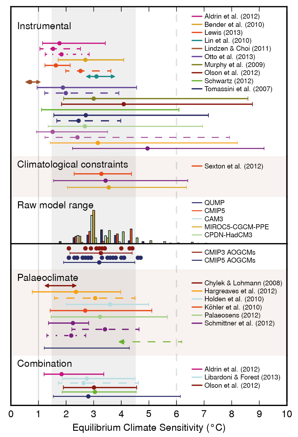
Estimates of equilibrium climate sensitivity from the recent IPCC report. The dots indicate the mean estimates, the horizontal lines the confidence intervals. Only studies new to this IPCC report are labelled.

Looking at projections is "only" the last few decades, how does it look for the entire instrumental record? People have estimated the climate sensitivity from the global warming observed until now. The equilibrium climate sensitivity indicates how much warming is expected on the long term for a doubling of the CO2 concentration. The figure to the right shows that several lines of evidence suggest that the equilibrium climate sensitivity is about 3. This value is not only estimated from the climate models, but also from climatological constraints (such as the Earth having escaped from [[snow-ball Earth]]), from the response to volcanoes and from a diverse range of paleo reconstructions of past changes in the climate. And newly Andrew Dessler estimated the climate sensitivity to be 3 based on decadal variability.

The outliers are the "instrumental" estimates. Not only do they scatter a lot and have large confidence intervals; that is to be expected because global warming has only increased the temperature by 1°C up to now. However, these estimates are on average also below 3. This is a reason to critically assess the climate models, climatological constraints and paleo reconstructions, but the most likely resolution would be that the outlier category, the "instrumental" estimates, are not accurate.

The term "instrumental" estimate refers to highly simplified climate models that are tuned to the observed warming. They need additional information on the change in CO2 (quite reliable) and on changes in atmospheric dust particles (so-called aerosols) and their influence on clouds (highly uncertain). The large spread suggests that these methods are not (yet) robust and some of the simplifications also seem to produce biases towards too low sensitivity estimates. That these estimates are on average below 3 is likely mostly due to such problems with the method, but it could also suggest that "the observations are running cold".

In this light, the paper discussed over at And Then There's Physics is interesting. The paper reviews the scientific literature on the relationship between how well climate models simulate a change in the climate for which we have good observations and which is important for the climate sensitivity (water vapour, clouds, tropical thunderstorms and ice) and the climate sensitivity these models have. It argues that:
the collective guidance of this literature [shows] that model error has more likely resulted in ECS underestimation.
Given that these "emergent constraint" studies find that the climate sensitivity from dynamic climate models may well be too low rather than too high, it makes sense to investigate whether the estimates from the "instrumental" category, the highly simplified climate models, are too low. One reason could be because we have underestimated the amount of surface warming.

The top panel (A) shows a measure for the mixing between the lower and middle troposphere (LTMI) over warm tropical oceans. The observed range is between the two vertical dashed lines. Every coloured dot is a climate model. Only the models with a high equilibrium climate sensitivity are able to reproduce the observed lower tropospheric mixing.
The lower panel(B) shows a qualitative summary of the studies in this field. The vertical line is the climate sensitivity averaged over all climate models. For the models that reproduce water vapour well this average is about the same. For the models that reproduce ice (cryosphere), clouds, tropical thunder storms (ITCZ) well the climate sensitivity is higher.

Concluding, climate models and further estimates of the climate sensitivity suggest that we may underestimate the warming of the surface temperature. This is certainly not conclusive, but there are many lines of evidence that climate change is going faster than expected as we will in further posts in this series: Arctic sea ice and snow cover, precipitation, sea level rise predictions, lake and river warming, etc. In combination the [[consilienceof evidence]] suggests at least that "the observations running cold" is something we need to investigate.

Looking at the way station measurements are made there are also several reasons why the raw observations may show too little warming. The station temperature record is rightly seen as a reliable information source, but in the end it is just one piece of evidence and we should consider all of the evidence.

There are so many lines of evidence for underestimating global warming that science historian Naomi Oreskes wondered if climate scientists had a tendency to "err on the side of least drama" (Brysse et al., 2013). Rather than such a bias, all these underestimates of the speed of climate change could also have a common cause: an underestimate of global warming.

I did my best to give a fair view of the scientific literature, but like for most posts in this series this topic goes beyond my expertise (station data). Thus a main reason to write these posts is to get qualified feedback. Please use the comments for this or write to me.


Related information

Gavin Schmidt wrote the same 2 years ago from a modellers perspective: On mismatches between models and observations.

Gavin Schmidt's TED talk: The emergent patterns of climate change and corresponding article.

Climate Scientists Erring on the Side of Least Drama

Why raw temperatures show too little global warming

First post in this series wondering about a cooling bias: Lakes are warming at a surprisingly fast rate

References

Cowtan, Kevin, Zeke Hausfather, Ed Hawkins, Peter Jacobs, Michael E. Mann, Sonya K. Miller, Byron A. Steinman, Martin B. Stolpe, and Robert G. Way, 2015: Robust comparison of climate models with observations using blended land air and ocean sea surface temperatures. Geophysical Research Letters, 42, 6526–6534, doi: 10.1002/2015GL064888.

Fasullo, John T., Benjamin M. Sanderson and Kevin E. Trenberth, 2015: Recent Progress in Constraining Climate Sensitivity With Model Ensembles. Current Climate Change Reports, first online: 16 August 2015, doi: 10.1007/s40641-015-0021-7.

Schmidt, Gavin A. and Steven Sherwood, 2015: A practical philosophy of complex climate modelling. European Journal for Philosophy of Science, 5, no. 2, 149-169, doi: 10.1007/s13194-014-0102-9.

Brysse, Keynyn, Naomi Oreskes, Jessica O’Reilly and Michael Oppenheimer, 2013: Climate change prediction: Erring on the side of least drama? Global Environmental Change, 23, Issue 1, February 2013, Pages 327–337, doi: 10.1016/j.gloenvcha.2012.10.008.

Sunday, August 30, 2015

Democracy is more important than climate change #WOLFPAC

I know, I know, this is comparing apples to oranges. This is a political post. I am thinking of a specific action I am enthusiastic about to make America a great democracy again: WOLFPAC is working to get a constitutional amendment to get money out of politics. If I had to chose between a mitigation sceptical WOLFPAC candidate and someone who accepts climate change, but is against this amendment, I would chose the mitigation sceptic.

Money is destroying American politics. Politicians need money for their campaigns. The politician with most money nearly always wins. This goes both ways; bribing the winner is more effective, but money for headquarters and advertisements sure help a lot to win. For the companies this is a good investment; the bribe is normally much smaller than the additional profit they make by getting contracts and law changes. Pure crony capitalism.

This is a cross-partisan issue. Republican presidential candidate Donald Trump boosted:
[W]hen you give, they do whatever the hell you want them to do. ... I will tell you that our system is broken. I gave to many people. Before this, before two months ago, I was a businessman. I give to everybody. When they call, I give. And you know what? When I need something from them, two years later, three years later, I call them. They are there for me. And that's a broken system.
For Democrat presidential candidate Bernie Sanders getting money out of politics is a priority issue. He will introduce "the Democracy Is for People constitutional amendment" and promises "that any Sanders Administration Supreme Court nominee will commit to overturning the disastrous Citizens United decision."

Bribery will not stop with an appeal to decency. It should be forbidden.

The WOLFPAC plan to get bribery forbidden sounds strong. They want to get a constitutional amendment to forbid companies to bribe politicians and want this amendment passed by the states, rather than Washington, because the federal politicians depend most on the corporate funding. They believe that state legislators believe stronger in their political ideals. This is also my impression in local politics as a student; also the politicians I did not agree with mostly seemed to believe in what they said. Once I even overheard a local politician passionately discussing a reorganization to improve services and employee moral, with his girlfriend in a train on a Saturday afternoon.

In Washington it is harder to win against lobbies who have much more money. At the state level election campaigns are cheaper, this makes the voice of the people stronger and a little money makes more impact. This makes it easier for WOLFPAC to influence the elections; try to get rid of politicians who oppose the amendment, reward the ones that work for it.

Even at the federal level there may actually be some possibilities. Corporations also compete with each other. They are thus more willing to fund campaigns that help themselves than campaigns that help all companies. In the most extreme case, if only one company would have to cough up all the money to keep money in politics, this company would be a lot less profitable than all the others that benefit from this "altruistic company". In other words, even if companies have a lot of money, you are not fighting against their entire war chest.

Almost all people are in favour of getting money out of politics. Thus a campaign in favour of it is much cheaper than one against. WOLFPAC was founded by the owner of The Young Turks internet news company, which has a reach that is comparable to the cable new channels. This guarantees that the topic will not go away and that time is on our side. Some politicians may like to ignore the amendment as long as they can, but will not dare to openly oppose such a popular proposal. With more and more states signing on, the movement becomes harder to ignore.

Wealthy individuals may well bribe politicians now, but be in favour of no one being able to do so. Just like someone can fly or drive a car while being in favour of changing the transport system so that this is no longer necessary.

It needs two thirds of the states (34) to call for a constitutional convention on a certain topic. The amendment that comes out of this then has to be approved by three quarter of the states. The beginning is hardest, but at the moment I am writing this, the main hurdle has already been taken: four states—Vermont, California, New Jersey and Illinois—have already called for a constitutional convention, see map at the top. In
Connecticut, Delaware, Hawaii, Maryland, Missouri and New Hampshire, the amendment already passed one of the houses. In many more the resolution has been introduced or approved in committees.


I would say this has a good chance of winning. It would feel so good to get this working. For America and for the rest of the world; given how dominant America is, a functioning US political system is important for everyone. It would probably also do a lot to heal the culture war in America, fuelled by negative campaigning. As such it could calm down the climate "debate", which is clearly motivated by politics and only pretends to worry about the integrity of science. The nasty climate "debate" is a social problem in the USA, which should be solved politically in the USA, no amount of science communication can do this.

A recent survey across 14 industrialised nations has found that Australia and Norway are the most mitigation sceptical countries. This does not hurt Norway because it has a working political system. A Norwegian politician could not point to a small percentage of political radicals to satisfy his donors. In a working political system playing the fool seriously hurts your reputation; it would probably even work better to honestly say you do this because you support fossil fuel companies. The political radicals at WUWT & Co. will not go away, but it is not a law that politicians use them as excuse.

[UPDATE. Politics in Australia also works, just a little slower, mitigation sceptical prime minister Tony Abbott toppled after two years by science accepting Malcolm Turnbull.]

Please have a look at the plan of WOLFPAC. I think it could work and that would be fabulous.


Monday, August 24, 2015

Karl Rove strategy #3: Accuse your opponent of your own weakness

Quite often a mitigation skeptic will present an "argument" that would make sense if the science side would make it, but makes no sense from their side. Classics would be dead African babies or being in it for the money.

A more person example would be Anthony Watts, the host of mitigation skeptical blog WUWT, claiming that I have a WUWT fixation. Fixation champion Anthony Watts who incites hatred of Michael E. Mann on a weekly if not daily basis. That I write about his cesspit occasionally makes sense given that Watts claims to doubt the temperature trend from station measurements; that is my topic. WUWT is also hard to avoid given that PR professional Watts calls his blog "The world's most viewed site on global warming and climate changes" to improve its standing with journalists and his blog is at least a larger one thus the immoral behavior of WUWT represents the mainstream of the political movement against mitigation.

You can naturally see this behavior as the psychological problem called [[projection]]:
Psychological projection is the act or technique of defending oneself against unpleasant impulses by denying their existence in oneself, while attributing them to others.

Political strategy

It is also a political strategy. One that works. It is strategy #3 on the list of USA Republican political strategist Karl Rove. If you see two groups basically making the same claim, it is hard to decide who is right. That requires going into the details, investing time and most people will not do that. They will simply select the version they like most and go on with their lives.

I must admit that I did not see a good way to respond the #3 nonsense and typically simply ignored it rationalizing that these people were anyway too radical, that communication with them is useless. However, that makes no sense, because communicating with the political extremists at WUWT & Co. never makes sense; it is futile to hope to convince them. You communicate with these people for the lurkers (if there are normal people around). For the lurkers it may be less clear who is wrong and for the lurkers it may be less clear that this is a pattern, a strategy.

Thus I was happy to finally have found a suggestion how to reply. Art Silverblatt—professor of Communication and Journalism—and colleagues have developed strategies to neutralize the strategies of Karl Rove. Their response strategy is to make clear to the pubic how strategy #3 works and deflect it with humor.

For example when Ronni Earle was attacked by Tom DeLay using strategy #3, his response strategy was:
Earle put the into perspective for the public, saying, "I find they often accuse others of doing what they themselves do.”

[Earle] chose to discuss the tactic in terms of how it denigrated the political process and, ultimately, the voters. "This is about protecting the integrity of our electoral system and I couldn't just ignore it."

Earle took a humorous approach, so that he wasn't thrown off-stride by the attacks.

"Being called vindictive and partisan by Tom DeLay is like being called ugly by a frog."
In the climate "debate" it is probably also a good idea to bring the discussion back to the facts. Our strong point is that we have science on our side. Try to make mitigations skeptics to stick to one point and debate this in detail, that exposes their weakest side. Point the lurkers to all their factual and thinking errors, debating tricks and attempts to change the topic.


Poor African babies

So how to respond next time someone claims that scientists doing their job to understand the climate system and how the climate is changing are killing African babies that need coal to survive? Explain that it is a typical strategy for political extremists to claim that other people do what they themselves do, that they do this to confuse the audience. That this endangers our open democratic societies and in the end our freedom and prosperity.

That the opposition to mitigation is delaying solving the problem and that this will kill many vulnerable people. Unfortunately, we do not only have nice people on this world, for some the impacts of climate change may the reason to want to delay solving the problem. Thus it is likely good to also note that the largest economic damages will be in the industrialized countries. That the reason we are wealthy and powerful is our investment in capital. That these investments have been made for the climate of the past. That the high input of capital means that industrialized societies are highly optimized and more easily disrupted.


I would also explain that in the current phase the industrialized world needs to build up renewable energy systems to drive the costs down. That no one expects poor countries to do this. Because many African countries have a very low population density, centralized power plants would need expensive distribution systems and ever cheaper renewable energy is often a good choice, especially in combination with cell phones. Building up a renewable energy system in the industrialized world would also reduce demand of fossil fuels on the world market and lower the prices for the global poor.


Any ideas to put more humor in this response? I have been living in Germany for too long.


Related reading

Denying reality may be nice on the short-term, but is not a viable long-term strategy, as Donald Trump's nomination shows: Believe me, the GOP needs to open itself to rational debate

Be aware that not everyone shares your values: Do dissenters like climate change?

How to talk with mitigation skeptics online: My immature and neurotic fixation on WUWT.

How to talk with someone you know in person about climate change: How to talk to uncle Bob, the climate ostrich.


* Solar power world wide figure by SolarGIS © 2011 GeoModel Solar s.r.o. This figure is licensed under the Creative Commons Attribution-Share Alike 3.0 Unported license.

Tuesday, August 11, 2015

History of temperature scales and their impact on the climate trends

Guest post by Peter Pavlásek of the Slovak Institute of Metrology. Metrology, not meteorology, they are the scientists that work on making measurements more precise by developing high accurate standards and thus make experimental results better comparable.

Since the beginning of climate observations temperature has always been an important quantity that needed to be measured as its values affected every aspect of human society. Therefore its precise and reliable temperature determination was important. Of course the ability to precisely measure temperature strongly depends on the measuring sensor and method. To be able to determine how precisely the sensor measures temperature it needs to be calibrated by a temperature standard. As science progressed with time new temperature scales were introduced and the previous temperature standards naturally changed. In the following sections we will have a look on the importance of temperature scales throughout the history and their impact on evaluation of historical climate data.

The first definition of a temperature standard was created in 1889. At the time thermometers were ubiquitous, and had been used for centuries; for example, they had been used to document ocean and air temperature now included in historical records. Metrological temperature standards are based on state transitions of matter (under defined conditions and matter composition) that generate a precise and highly reproducible temperature value. For example, the melting of ice, the freezing of pure metals, etc. Multiple standards can be used as a base for a temperature scale by creating a set of defined temperature points along the scale. An early definition of a temperature scale was invented by the medical doctor Sebastiano Bartolo (1635-1676), who was the first to use melting snow and the boiling point of water to calibrate his mercury thermometers. In 1694 Carlo Renaldini, mathematician and engineer, suggested using the ice melting point and the boiling point of water to divide the interval between these two points into 12 degrees, applying marks on a glass tube containing mercury. Reamur divided the scale in 80 degrees, while the modern division of roughly 100 degrees was adopted by Anders Celsius in 1742. Common to all the scales was the use of phase transitions as anchor points, or fixed points, to define intermediate temperature values.

It is not until 1878 that the first sort of standardized mercury-in-glass thermometers were introduced as an accompanying instrument for the metre prototype, to correct from thermal expansion of the length standard. These special thermometers were constructed to guarantee reproducibility of measurement of a few thousandths of a degree. They were calibrated at the Bureau International des Poids et Mesures (BIPM), established after the recent signature of the Convention du Metre of 1875. The first reference temperature scale was adopted by the 1st Conférence générale des poids et measures ( CGPM) in 1889. It was based on constant volume gas thermometry, and relied heavily on the work of Chappius at BIPM, who had used the technique to link the readings of the very best mercury-in-glass thermometers to absolute (i.e. thermodynamic) temperatures.

Meanwhile, the work of Hugh Longbourne Callendar and Ernest Howard Griffiths on the development of platinum resistance thermometers (PRTs) lay the foundations for the first practical scale. In 1913, after a proposal from the main Institutes of metrology, the 5th CGPM encouraged the creation of a thermodynamic International Temperature Scale (ITS) with associated practical realizations, thus merging the two concepts. The development was halted by the World War I, but the discussions resumed in 1923 when platinum resistance thermometers were well developed and could be used to cover the range from –38 °C, the freezing point of mercury, to 444.5 °C, the boiling point of sulphur, using a quadratic interpolation formula, that included the boiling point of water at 100 °C. In 1927 the 7th CGPM adopted the International Temperature Scale of 1927 that even extended the use of PRTs to -183 °C. The main intention was to overcome the practical difficulties of the direct realization of thermodynamic temperatures by gas thermometry, and the scale was a universally acceptable replacement for the various existing national temperature scales.

In 1937 the CIPM established the Consultative Committee on Thermometry (CCT). Since then the CCT has taken all initiatives in matter of temperature definition and thermometry, including, in the recent years, issues concerning environment, climate and meteorology. It was in fact the CCT that in 2010, shortly after the BIPM-WMO workshop on “Measurement Challenges for Global Observing Systems for Climate Change Monitoring” submitted the recommendation CIPM (T3 2010), encouraging National Metrology Institutes to cooperate with the meteorology and climate communities for establishing traceability to those thermal measurements of importance for detecting climate trends.

The first revision of the 1927 ITS took place in 1948, when extrapolation below the oxygen point to –190 °C was removed from the standard, since it had been found to be an unreliable procedure. The IPTS-48 (with “P” now standing for “practical”) extended down only to –182.97 °C. It was also decided to drop the name "degree Centigrade" for the unit and replace it by degree Celsius. In 1954 the 10th CGPM finally adopted a proposal that Kelvin had made back one century before, namely that the unit of thermodynamic temperature to be defined in terms of the interval between the absolute zero and a single fixed point. The fixed point chosen was the triple point of water, which was assigned the thermodynamic temperature of 273.16 °K or equivalently 0.01 °C and replaced the melting point of ice. Work continued on helium vapour pressure scales and in 1958 and 1962 the efforts were concentrated at low temperatures below 0.9 K. In 1964 the CCT defined the reference function “W” for interpolating the PRTs readings between all new low temperature fixed points, from 12 K to 273,16 K and in 1966 further work on radiometry, noise, acoustic and magnetic thermometry made CCT preparing for a new scale definition.

In 1968 the second revision of the ITS was delivered: both thermodynamic and practical units were defined to be identical and equal to 1/273.16 of the thermodynamic temperature of the triple point of water. The unit itself was renamed "the kelvin" in place of "degree Kelvin" and designated "K" in place of "°K". In 1976 further consideration and results at low temperatures between 0.5 K and 30 K were included in the Provisional Temperature Scale, EPT-76. Meanwhile several NMIs continued the work to better define the fixed points values and the PRT’s characteristics. The International Temperature Scale of 1990 (ITS-90) came into effect on 1 January 1990, replacing the IPTS-68 and the EPT-76 and is still today adopted to guarantee traceability of temperature measurements. Among the main features of ITS-90, with respect to the 1968 one, is the use of the triple point of water (273.16 K), rather than the freezing point of water (273.15 K), as a defining point; it is in closer agreement with thermodynamic temperatures; it has improved continuity and precision.

It follows that any temperature measurement made before 1927 is impossible to trace to an international standard, except for a few nations with a well-defined national definition. Later on, during the evolution of both the temperature unit and the associated scales, changes have been introduced to improve the realization and measurement accuracy.

With each redefinition of the practical temperature scale since the original scale of 1927, the BIPM published official transformation tables to enable conversion between the old and the revised temperature scale (BIPM. 1990). Because of the way the temperature scales have been defined, they really represent an overlap of multiple temperature ranges, each of which may have their own interpolating instrument, fixed points or mathematical equations describing instrument response. A consequence of this complexity is that no simple mathematical relations can be constructed to convert temperatures acquired according to older scales into the modern ITS90 scale.

As an example of the effect of temperature scales alternations let us examine the correction of the daily mean temperature record at Brera, Milano in Italy from 1927 to 2010, shown in Figure 1. The figure illustrates the consequences of the temperature scale change and the correction that needed to be applied to convert the historical data to the current ITS-90. The introduction of new temperature scales in 1968 and 1990 is clearly visible as discontinuities in the magnitude of the correction, with significantly larger corrections for data prior to 1968. As expected from Figure 1, the cycling follows the seasonal changes in temperature. The higher summer temperatures require a larger correction.


Figure 1. Example corrections for the weather station at Brera, Milano in Italy. The values are computed for the daily average temperature. The magnitude of the correction cycles with the annual variations in temperature: the inset highlights how the warm summer temperatures are corrected much more (downward) than the cool winter temperatures.

For the same reason the corrections will differ between locations. The daily average temperatures at the Milano station typically approaches 30 °C on the warmest summer days, while it may fall slightly below freezing in winter. In a different location with larger differences between typical summer and winter temperature the corrections might oscillate around 0 °C, and a more stable climate might see smaller corrections overall: at Utsira, a small island off the south-western coast of Norway the summertime corrections are typically 50% below the values for Brera. To better see the magnitude of corrections for specific historical temperatures the Figure 2 is provided.


Figure 2. The corrections in °C that need to be applied to a certain historical temperatures in the range form -50 °C up to +50 °C with regard to the time period the historical data were measured.

The uncertainty in the temperature readings from any individual thermometer is significantly larger than the corrections presented here. Furthermore, even for the limited timespan since 1927 a typical meteorological weather station has seen many changes which may affect the temperature readings. Examples include instrument replacement; instrument relocations; screens may be rebuilt, redesigned or moved; the schedule for readings may change; the environment close to the station may become more densely populated and therefore enhance the urban heat island effect; and manually recorded temperatures may suffer from unconscious observer bias (Camuffo, 2002; Bergstrøm and Moberg, 2002; Kennedy, 2013). Despite the diligent quality control employed by meteorologists during the reconstruction of long records, every such correction also has an uncertainty associated with it. Thus, for an individual instrument, and perhaps even an individual station, the scale correction is insignificant.

On the other hand, more care is needed for aggregate data. The scale correction represents a bias which is equal for all instruments, regardless of location and use, and simply averaging data from multiple sources will not eliminate it. The scale correction is smaller than, but of the same order of magnitude as the uncertainty components claimed for monthly average global temperatures in the HadCRUT4 dataset (Morice et al., 2012). To evaluate the actual value of the correction for the global averages would require a recalculation of all the individual temperature records. However, the correction does not alter the warming trend: if anything it would exacerbate it slightly. Time averaging or averaging multiple instruments has been claimed to lower temperature uncertainty to around 0.03 °C (for example in Kennedy (2013) for aggregate temperature records of sea surface temperature). To be credible such claims for the uncertainty need to consider the scale correction in our opinion.

Scale correction for temperatures earlier than 1927 is harder to assess. Without an internationally accepted and widespread calibration reference it is impossible to construct a simple correction algorithm, but there is reason to suspect that the corrections become more important for older parts of the instrumental record. Quantifying the correction would entail close scrutiny of the old calibration practices, and hinges on available contemporary descriptions. Conspicuous errors can be detected, such as the large discrepancy which Burnette et al. found in 1861 from records at Fort Riley, Kansas (Burnette et al., 2010). In that case the decision to correct the dubious values was corroborated by metadata describing a change of observer: however, this also illustrates the calibration pitfall when no widespread temperature standard was available. One would expect that many more instruments were slightly off, and the question is whether this introduced a bias or just random fluctuations which can be averaged away when producing regional averages.

Whether the relative importance of the scale correction increases further back in time remains an open question. The errors from other sources such as the time schedule for the measurements also become more important and harder to account for, such as the transformation from old Italian time to modern western European time described in (Camuffo, 2002).

This brief overview of temperature scales history has shown what an impact these changes have on historical temperature data. As it was discussed earlier the corrections originating from the temperature scale changes is small when compared with other factors. Even when the values of the correction may be small it doesn’t mean it should be ignored as their magnitude are far from negligible. More details about this problematic and the conversion equation that enables to convert any historical temperature data from 1927 up to 1989 to the current ITS-90 can be found in the publication of Pavlasek et al. (2015).


Related reading

Why raw temperatures show too little global warming

Just the facts, homogenization adjustments reduce global warming

References

Camuffo, Dario, 2002: Errors in early temperature series arising from changes in style of measuring time, sampling schedule and number of observations. Climatic change, 53, pp. 331-352.

Bergstrøm, H. and A. Moberg, 2002: Daily air temperature and pressure series for Uppsala (1722-1998). Climatic change, 53, pp. 213-252.

Kenndy, John J., 2013: A review of uncertainty in in situ measurements and data sets of sea surface temperature. Reviews of geophysics, 52, pp. 1-32.

Morice, C.P., et al., 2012: Quantifying uncertainties in global and regional temperature change using an ensemble of observational estimates: The HaddCRUT4 data set. Journal of geophysical research, 117, pp. 1-22.

Burnette, Dorian J., David W. Stahle, and Cary J. Mock, 2010: Daily-Mean Temperature Reconstructed for Kansas from Early Instrumental and Modern Observations. Journal of Climate, 23, pp. 1308-1333.

Pavlasek P., A. Merlone, C. Musacchio, A.A.F. Olsen, R.A. Bergerud, and L. Knazovicka, 2015: Effect of changes in temperature scales on historical temperature data. International Journal of Climatology, doi: 10.1002/joc.4404.

Friday, July 17, 2015

Lakes are warming at a surprisingly fast rate


Map with lake temperature trends. As so often the trend is strongest in the mid-latitudes of the Northern Hemisphere. Two seasons are used to minimize cloud blockage: JAS (July, August & September) and JFM (January, February & March) for the dry season.

Many changes in the climate system go faster than expected, which fits to my hunch that the station temperature trend may have a cooling bias. The coming time I would like to blog about a few example changes. This first post is about lakes and rivers, their temperature changes and changes in the date they freeze and the date the ice breaks up. In this case it is hard to say whether this goes faster than expected, because there is not much research on this, but the temperature changes sure are surprisingly fast.

We will see more research on this in future. There is now a Global Lake Temperature Collaboration (GLTC), which is collecting and analyzing lake temperatures. It is easy to complain about the weather services and how they keep on making changes to the meteorological networks and fail to share many important observational datasets (and I will keep complaining), but at least they have systematically made such historical observations. For other observations, such a lake temperatures and especially ecological datasets it is much harder to obtain long and stable observations lacking institutional support. Now going into the century of climate change this institutional failure becomes even more problematic. I feel it should be part of the international climate change treaties to set up organizations that can provide long term, well-documented and climate quality stable measurements of a large range of environmental systems.

One of the reasons to found the Global Lake Temperature Collaboration was a scientific article by Schneider and Hook in 2010. It analyzed the temperature trends of lakes using thermal infra-red satellite images ([[AVHRR]] and [[ATSR]]). Between 1985 and 2009 the satellite lake temperatures increased by 1.13°C, which they report is more than the regional air temperature increases. For comparison this amounts to 4.5°C per century; see graph below. This is stronger than the land temperatures, although one would expect less warming of the lakes. For the same period the Northern Hemisphere temperature of Berkeley Earth increased by 3.9°C per century.


Trend in lake temperature anomalies. This is an average over all 113 water bodies that were large enough and had at least 15 years of data. The trend over the period 1985 to 2009 is 4.5±1.1°C per century.

Satellite data is great for their global overview (see graph at the top of this post), but are tricky when it comes to trends. Trend estimates from satellite data are difficult due to degradation of the instruments in a harsh space environment, changes in the orbit and height of the satellite, while at the same time the limited life span of satellites means that the instruments are regularly replaced and technological improvement often lead to new designs. All this happens while the small number of satellites means that there is minimal redundancy to study such data problems. Schneider and Hook (2010) did their best to study such data problems, used data from seasons with few clouds, so that the satellite can see the lakes more often. They compared their data with surface observations and found only small biases between the satellites and no indications of trend biases. And they used night-time observations to reduce the influence of orbital drift.

Still an astonishing outlier trend from satellite data calls for ground validation (in situ measurements). The GLTC now provides a dataset with both satellite and in-situ lake temperature measurements. The paper describing the dataset is out now (Sharma et al., 2015). The paper analyzing the trends has still to be published, but Philipp Schneider of the GLTC wrote to me that the in-situ trend is similar. Further papers explaining the trends are in preparation.

At the moment it is not clear yet what is the reason for the stronger increase. Many lakes are close to the Arctic, thus it could be ice albedo feedback for Northern lakes. The summer surface temperature of Lake Superior over the interval 1979 - 2006 has, for example, increased by 11±6°C per century, faster than regional atmospheric warming. This is thought to be due a reduction in the albedo of the lakes due to a reduction in ice cover (Austin and Colman, 2007). The air in the Arctic is also warming faster than elsewhere. Changes in the observations are naturally also possible — as always — and the land surface temperature trend might also be underestimated.

Stronger insolation may especially heat lakes, which typically reflect less solar radiation than the land surface. This may especially be important for the recent decades in the industrialised countries, where air pollution has been reduced considerably.

Surface temperatures may change due to less mixing with deep cold water: as the top temperatures warm more the warm surface water mixes less well with the deep cold and dense water and reductions in the wind speed can reduce mixing (Butcher et al., 2015). Also changes in the transparency of the water can influence where the solar warming ends up (Butcher et al., 2015).

In other words, no observation is ever completely straight forward and the air temperature is just one factor influencing lake water temperatures. Just like with station measurements, you always need to study which part of the changes in the raw observations is the part you are interested in.

On the other hand, because more of the additional greenhouse warming goes into evaporation rather than to warming, the warming of the air over land is expected to be stronger than the lake water temperatures. Butcher and colleagues (2015) estimate that the surface water temperature increases are only about 77% of increase in average air temperature change. Previously Schmidt and colleagues (2014) estimated this to be between 70 to 85%.

Freezing and melting of lakes and rivers

The lake temperature observations are unfortunately not very long. To put their warming into perspective there are also observations of the freezing and breakup dates of lakes and rivers. These sometimes go back many centuries. Magnuson and colleagues (2000) have gathered 39 observational dataset on lakes and rivers with more than 150 years of data. They found that all but one of them showed later freezing dates and earlier breakup dates. The freeze dates are 5.8 days per century later and the breakup dates are 6.5 days per century earlier. This is comparable to a warming of the regional air temperature of about 1.2°C (2°F) per century, but with a large confidence interval. For comparison, the Berkeley Earth dataset shows a warming of the NH land temperatures for the same period between 1846 and 1995 of 0.67°C per century. For this comparison it should be reminded that these rivers and lakes are in high latitude regions that warm more.


Time series of freeze and breakup dates from selected Northern Hemisphere lakes and rivers (1846 to 1995). Data were smoothed with a 10-year moving average. Figure 1 from Magnuson (2002).

For one dataset they mention a small non-climatic influence (a power plant) and one dataset (a harbor) is excluded because of its much stronger trend. Magnuson and colleagues seem confident that warm waste water is not the reason for the trends in the other series, but do not explicitly write about that in their 4-page Science article.


Melting lakes showing a clear contrast between ice and water. This makes is relatively easy to use historical aircraft and satellite observations. Figure 5 from Duguay et al. (2003).
The advantage of such datasets is that they provide yearly information, that the observations are often long and that they are relatively precise. For the recent decades, the observations can be made for a large number of lakes from space. These freezing and breakup dates are also nicely determined by the temperature averaged over a longer period, which removes a lot of variability: Freezing is determined by the temperature in the last two months before the event.

What complicates matters is that snow isolates the ice and slows down freezing and thawing. Thus the ice breakup of lakes is also influenced by snow on top of the ice. Also the depth of the lake is important; deeper lakes thaw later (Duguay and colleagues, 2003). The breakup date of rivers is also determined by the timing and amount of spring river run-off.

Concluding. Lake temperature are rising fast over the last decades, likely faster than the air temperatures, while one would expect that lakes warm slower because more heat goes into evaporation. This could be in part due to an albedo feedback or due to more sunshine from reductions in air pollution during these decades. Furthermore, also the length of the period that lakes and rivers are frozen decreases rapidly since 1850. Converting this in a temperature signal introduces a large uncertainty, but also this temperature increase seems to be faster than the current estimates of land surface temperature increases.

Now if I were a political activist, I would call climate science a hoax or claim that all scientists are stupid. Just listen to lonely brilliant Galileo me, forget science, the oceans will boil soon.

But, well, I am sorry for being such a scientist, I would just say, that we found something very interesting. Apparent discrepancies help one to understand a problem better. Only once we understand the warming of the lakes better can we know whether climate science was wrong.

As will be the case for most of this blog series on faster changes, the topic of this post goes beyond my expertise. Thus if anyone knows of good studies on this topic, I would be very grateful if you could leave a comment or would write me. Especially if anyone knows of comparisons between air and water temperature trends or between models and observations for lake and river temperatures or their ice cover. There are a number of interesting papers coming up, thus I will probably have to write an update in a few months.


Related resources

Climate Central reports on a new study (December 2015) on global lake temperature changes.

John Lenters (coordinator of the GLTC) at Nature's Scientific Data blog: Author’s Corner: Are lakes warming?

Global Lake Temperature Collaboration

Why raw temperatures show too little global warming

A recent study shows that since 1970 the ocean heat content of the upper 700m has increased 15% more than climate models have predicted.

Chris Mooney has an interesting piece in the Washington Post on related snow cover observations: Northern Hemisphere snow cover is near record lows. Here’s why that should worry you.

More scientific articles on lake ice by the group of John Magnuson.

The river and like ice phenology database: Benson, B. and J. Magnuson. 2000, updated 2012. Global lake and river ice phenology database. Boulder, Colorado USA: National Snow and Ice Data Center. doi: 10.7265/N5W66HP8.

References

Austin, J. A. and S. M. Colman, 2007: Lake Superior summer water temperatures are increasing more rapidly than regional air temperatures: A positive ice-albedo feedback, Geophysical Research Letters, 34, art. no. L06604, doi: 10.1029/2006GL029021.

Butcher, Jonathan B., Daniel Nover, Thomas E. Johnson, and Christopher M. Clark, 2015: Sensitivity of lake thermal and mixing dynamics to climate change. Climatic Change, March 2015, 129, Issue 1-2, pp 295-305, doi: 10.1007/s10584-015-1326-1.

Duguay, Claude R., Greg M. Flato, Martin O. Jeffries, Patrick Ménard, Kim Morris, and Wayne R. Rouse, 2003: Ice-cover variability on shallow lakes at high latitudes: model simulations and observations. Hydrological Processes, 17, pp. 3465-3483, doi: 10.1002/hyp.1394.

Magnuson, John J., Dale M. Robertson, Barbara J. Benson, Randolf H. Wynne, David M. Livingstone, Tadashi Arai, Raymond A. Assel, Roger B. Barry, Virginia Card, Esko Kuusisto, Nick G. Granin, Terry D. Prowse, Kenton M. Stewart, and Valery S. Vuglinski, 2000: Historical trends in lake and river ice cover in the Northern Hemisphere. Science, 289, pp. 1743-1746, doi: 10.1126/science.289.5485.1743.

Schmid, Martin, Stefan Hunziker, and Alfred Wüest , 2014: Lake surface temperatures in a changing climate: a global sensitivity analysis. Climatic Change, 124, pp. 301–315, doi: 10.1007/s10584-014-1087-2.

Schneider, Philipp, and Simon J. Hook, 2010: Space observations of inland water bodies show rapid surface warming since 1985. Geophysical Research Letters, 37, art. no. L22405, doi: 10.1029/2010GL045059.

Schneider, Philipp and Simon J. Hook, 2012: Global Trends of Lake Surface Temperatures Observed From Space. Geophysical Research Abstracts, 14, EGU2012-2858, EGU General Assembly 2012.

Schneider, Philipp, Simon J. Hook, Derek K. Gray, Jordan S. Read, Stephanie E. Hampton, Catherine M. O’Reilly, Sapna Sharma, and John D. Lenters, 2013: Global lake warming trends derived from satellite and in situ observations. Geophysical Research Abstracts, 15, EGU2013-2235, EGU General Assembly 2013.