Showing posts with label parallel measurements. Show all posts

Monday, March 21, 2016

Cooling moves of urban stations


It has been studied over and over again, in very many ways: in global temperature datasets urban stations have about the same temperature trend as surrounding rural stations.

There is also massive evidence that urban areas are typically warmer than their surroundings. For large urban areas the Urban Heat Island (UHI) effect can increase the temperature by several degrees Celsius.

A constant higher temperature due to the UHI does not influence temperature changes. However, when cities grow around a weather station, this produces an artificial warming trend.

Why don’t we see this in the urban stations of the global temperature collections? There are several reasons; the one I want to focus on in this post is that stations do not stay at the same place.

Urban stations are often relocated to better locations, more outside of town. It is common for urban stations to be moved to airports, especially when meteorological offices are moved to the airport to assist in airport safety. Also when meteorological offices can no longer pay the rent in the city center, they are forced to move out and take the station with them. When urban development makes the surrounding unsuited or when a volunteer observer retires, the station has to move, it makes sense to then search for a better location, which will likely be in a less urban area.

Relocations are nearly always the most frequent reason for inhomogeneities. For example, Manola Brunet and colleagues (2006) write about Spain:
“Changes in location and setting are the main cause of inhomogeneities (about 56% of stations). Station relocations have been common during the longest Spanish temperature records. Stations were moved from one place to another within the same city/town (i.e. from the city centre to outskirts in the distant past and, more recently, from outskirts to airfields and airports far away from urban influence) and from one setting (roofs) to another (courtyards).”
Since relocations of that kind are likely to result in a cooling, the Parallel Observations Science Team (ISTI-POST) wants to have a look at how large this effect is. As far as we know there is no overview study yet, but papers on the homogenization of a station network often report on adjustments made for specific inhomogeneities.

We, that is mainly Jenny Linden of Mainz University, had a look in the scientific literature. Let’s start in China were urbanization is strong and can be clearly seen in the raw data of many stations. They also have strong cooling relocations. The graph below from Wenhui Xu and colleagues (2013) shows the distribution of breaks that were detected (and corrected) with statistical homogenization for which the station history indicated that they were caused by relocations. Both the minimum and the maximum temperature cool by a few tenth of a degree Celsius due to the relocations.


The distribution of the breaks that were due to relocations for the maximum temperature (left) and minimum temperature (right). The red line is a Gaussian distribution for comparison.


Going more in detail, Zhongwei Yan (2010) and colleagues studied two relocations in Beijing. They found that the relocations cooled the observations by −0.81°C and −0.69°C. Yuan-Jian Yang and colleagues (2013) find a cooling relocation of 0.7°C in the data of Hefei. Clearly for single urban stations, relocations can have a large influence.

Fatemeh Rahimzadeh and Mojtaba Nassaji Zavareh (2014) homogenized the Iranian temperature observations and observed that relocations were frequent:
“The main non-climatic reasons for non-homogeneity of temperature series measured in Iran are relocation and changes in the measuring site, especially a move from town to higher elevations, due to urbanization and expansion of the city, construction of buildings beside the stations, and changes in vegetation.”
They show an example with 5 stations where one station (Khoramabad) has a relocation in 1980 and another station (Shahrekord) has two relocation in 1980 and 2002. These relocations have a strong cooling effect of 1 to 3 degrees Celsius.


Temperature in 5 stations in Iran, including their adjusted series.


The relocations do not always have a strong effect. Margarita Syrakova and Milena Stefanova (2009) do not find any influence of the inhomogeneities on the annual mean temperature averaged over Bulgaria. This while “Most of the inhomogeneities were caused by station relocations… As there were no changes of the type of thermometers, shelters and the calculation of the daily mean temperatures, the main reasons of inhomogeneities could be station relocations, changes of the environment or changes of the station type (class).

In Finland, Norway, Sweden and the UK the relocations produced a cooling bias of -0.11°C and relocations appear to be the most common cause of inhomogeneities (Tuomenvirta, 2001). The table below summarises the breaks that were found and what the reasons for them were if this was known from the station histories. They write:
“[Station histories suggest] that during the 1930s, 1940s and 1950s, there has been a tendency to move stations from closed areas in growing towns to more open sites, for example, to airports. This can be seen as a counter-action to increasing urbanization.”


Table with the average bias of inhomogeneities found in Finland, Sweden, Norway and the UK in winter (DJF), spring (MAM), summer (JJA) and autumn (SON) and in the yearly average. Changes in the surrounding, such as urbanization or micro-siting changes, made the temperatures higher. This was counteracted by more frequent cooling biases from changes in the thermometers and the screens used to protect the thermometers, by relocations and by changes in the formula used to compute the daily mean temperature.


Concluding, relocations are a frequent type of inhomogeneity. They produce a cooling bias. For urban stations the cooling can be very large. For the average over a region, the values are smaller, but especially because they are so common, they will have most likely a clear influence on global warming in raw temperature observations.

Future research

One problem with studying relocations is that they are frequently accompanied by other changes. Thus you can study them in two ways: study only relocations where you know that no other changes were made or study all historical relocations whether there was another change or not.

The first set-up allows us to characterize the relocations directly, to understand the physical consequences to move for example a station from the center of a city / village to the airport. In this way the differences are not subject to other changes specific to a network. So, the results can be easily compared between regions. The problem is that only a part of the parallel measurements available satisfy these strict conditions.

Conversely, for the second design (taking all historical relocations, also when they have another change) the characterization of the bias will be limited to the datasets studied and we will need a large sample to say something about the global climate record. But on the other hand, we can also analyze more data this way.

There are also two possible sources of information. The above studies relied on statistical homogenization comparing a candidate station to its neighbors. All you need to know for this is which inhomogeneities belong to a relocation. A more direct way to study these relocations is by using parallel measurements at both locations. This is especially helpful to study changes in the variability around the mean and in weather extremes. That is where the Parallel Observation Science Team (ISTI-POST) comes into play.

It is also possible to study specific relocations. The relocation of stations to airports was an important transition, especially around the 1940s. This temperature change is likely large and this transition quite frequent and well documented. One could focus on urban stations or on village stations, rather than studying all stations.

One could make a classification of the micro and macro siting before and after the relocation. For micro-siting the Michel Leroy (2010) classification could be interesting; as far as I know this classification has not been validated yet, we do not know how large the biases of the 5 categories are and how well-defined these biases are. Ian Stewart and Tim Oke (2012) have made a beautiful classification of the local climate zones of (urban) areas, which can also be used to classify the surrounding of stations.


Example of various combinations of building and land use of the local climate zones of Stewart and Oke.


There are many options and what we choose will also depend on what kind of data we can get. Currently our preference is to study parallel data with identical instrumentation at two locations, to understand the influence of the relocation itself as well as possible. In addition to study the influence on the mean, we are gathering data on the break sizes found by statistical homogenization for breaks due to relocations. The station histories (metadata) are crucial for this in order to clearly assign breakpoints to relocation activities. It will also be interesting to compare those two information sources where possible. This may become one study or two depending on how involved the analysis will become.

This POST study is coordinated by Alba Guilabert and Jenny Linden and Manuel Dienst are very active. Please contact one of us if you would like to be involved in a global study like this and tell us what kind of data you would have. Also if anyone knows of more studies reporting the size of inhomogeneities due to relocations, please let us know. I certainly have seen more such tables at conferences, but they may not have been published.


Related reading

Parallel Observations Science Team (POST) of the International Surface Temperature Initiative (ISTI).

The transition to automatic weather stations. We’d better study it now.

Changes in screen design leading to temperature trend biases.

Early global warming.

Why raw temperatures show too little global warming.

References

Brunet M., O. Saladie, P. Jones, J. Sigró, E. Aguilar, et al., 2006: The development of a new daily adjusted temperature dataset for Spain (SDATS) (1850–2003). International Journal of Climatology, 26, pp. 1777–1802, doi: 10.1002/joc.1338.
See also: a case-study/guidance on the development of long-term daily adjusted temperature datasets.

Leroy, M., 2010: Siting classifications for surface observing stations on land. In WMO Guide to Meteorological Instruments and Methods of Observation. "CIMO Guide", WMO-No. 8, Part I, Chapter 1, Annex 1B.

Rahimzadeh, F. and M.N. Zavareh, 2014: Effects of adjustment for non‐climatic discontinuities on determination of temperature trends and variability over Iran. International Journal of Climatology, 34, pp. 2079-2096, doi: 10.1002/joc.3823.

Stewart, I.D. and T.R. Oke, 2012: Local climate zones for urban temperature studies. Bulletin American Meteorological Society, 93, pp. 1879–1900, doi: 10.1175/BAMS-D-11-00019.1.
See also the World Urban Database.

Tuomenvirta, H., 2001: Homogeneity adjustments of temperature and precipitation series - Finnish and Nordic data. International Journal of Climatology, 21, pp. 495-506, doi: 10.1002/joc.616.

Xu, W., Q. Li, X.L. Wang, S. Yang, L. Cao, and Y. Feng, 2013: Homogenization of Chinese daily surface air temperatures and analysis of trends in the extreme temperature indices. Journal Geophysical Research Atmospheres, 118, doi: 10.1002/jgrd.50791.

Syrakova M. and Stefanova M., 2009: Homogenization of Bulgarian temperature series. International. Journal Climatology, 29, pp. 1835-1849, doi: 10.1002/jov.1829.

Yan ZW; Li Z; Xia JJ. 2014. Homogenisation of climate series: The basis for assessing climate changes. Science China: Earth Sciences, 57, pp 2891-2900, doi: 10.1007/s11430-014-4945-x.

* Photo at the top "High Above Sydney" by Taro Taylor used with a Attribution-NonCommercial 2.0 Generic (CC BY-NC 2.0) license.

Thursday, February 11, 2016

Early global warming

How much did the world warm during the transition to Stevenson screens around 1900?


Stevenson screen in Poland.

The main global temperature datasets show little or no warming in the land surface temperature and the sea surface temperature for the period between 1850 and 1920. I am wondering whether this is right or whether we do not correct the temperatures enough for the warm bias of screens that were used before the Stevenson screen was introduced. This transition mostly happened in this period.

This is gonna be a long story, but it is worth it. We start with the current estimates of warming in this period. There is not much data on how large the artificial cooling due to the introduction of Stevenson screens is, thus we need to understand why thermometers in Stevenson screens record lower temperatures than before to estimate how much warming this transition may have hidden. Then we compare this to the corrections NOAA makes for the introduction of the Stevenson screen. Also other changes in the climate system suggest there was warming in this period. It is naturally interesting to speculate what this stronger early warming may mean for the causes of global warming.

No global warming in main datasets

The figure below with the temperature estimates of the four main groups show no warming for the land temperature between 1850 and 1920. Only Berkeley and CRUTEM start in 1850, the other two later.

If you look at the land temperatures plotted by Berkeley Earth themselves there is actually a hint of warming. The composite figure below shows all four temperature estimates for their common area for the best comparison, while the Berkeley Earth figure is interpolated over the entire world and thus sees Arctic warming more, which was strong in this period, like it again was strong in recent times. Thus there was likely some warming in this period, mainly due to the warming Arctic.


The temperature changes of the land according to the last IPCC report. My box.

In the same period the sea surface temperature was even cooling a little according to HadSST3 shown below.


The sea surface temperature of the four main groups and night marine air temperature from the last IPCC report. I added the red box to mark the period of interest.

Also the large number of climate models runs produced by the Coupled Model Intercomparison Project (CIMP5), colloquial called IPCC models, do not show much warming in our period of interest.


CMIP5 climate model ensemble (yellow lines) and its mean (red line) plotted together with several instrumental temperature estimates (black lines). Figure from Jones et al. (2013) with our box added to emphasize the period.

Transition to Stevenson screens

In early times temperature observations were often made in unheated rooms or in window screens of such rooms facing poleward. These window screens protected the expensive thermometers against the weather and increasingly also against direct sun light, but a lot of sun could get onto the instrument or the sun could heat the wall beneath the thermometer and warm air would rise up.


A Wild screen (left) and a Stevenson screen in Basel, Switzerland.
When it was realised that these measurements have a bias, a period with much experimentation ensued. Scientists tried stands (free standing vertical boards with a little roof that often had to be rotated to avoid sun during sunrise and -fall), shelters of various sizes that were open to the poles and to the bottom, screens of various sizes, sometimes near the shade of a wall, but mostly in gardens and pagoda huts that could have been used for a tea party.

The more open a screen is, the better the ventilation, which likely motived earlier more open designs, but this also leads to radiation errors. In the end the Stevenson screen became the standard, which protects the instrument from radiation from all sides. It is made of white painted wood and has a measurement chamber mounted on a wood frame, it typically has a double board roof and double Louvred walls to all sides. Initially it sometimes did not have a bottom, but later had slanted boards at the bottom.

The first version [[Stevenson screen]] was crafted in 1864 in the UK, the final version designed in 1884. It is thought that most countries switched to Stevenson screens before 1920, but some countries were later. For example, Switzerland made the transition from Wild screens to Stevenson screens in the 1960s. The Belgium Station Uccle changed their half open shelter to a Stevenson screen in 1983. The rest of Belgium in the 1920s.


Open shelter (at the front) and two Stevenson screens (in the back) at the main office of the Belgium weather service in Uccle.

Radiation error

The schematic below shows the main factors influencing the radiation error. Solar radiation makes the observed maximum temperatures too warm. This can be direct radiation or radiation scattered via clouds or the (snow covered) ground. The sun can also heat the outside of a not perfectly white screen, which then warms the air flowing in. Similarly the sun can heat the ground, which then may radiate towards the thermometer and screen. However, the lack of radiation shielding also makes the minimum temperature too low when the thermometer radiates infrared radiation into the cold sky. This error is largest on dry cloudless nights and small when the sky radiates back to the thermometer, which happens when the sky is cloudy and the absolute humidity is high, which reduces the net infrared radiative cooling. The radiation error is largest when there is not much ventilation, which in most cases need wind. The direct radiation effects are smaller for smaller thermometers.


Schematic showing the various factors that can influence the radiation error of a temperature sensor.

From our understanding of the radiation error, we would thus expect the bias in the day-time maximum temperature to be large where the sun is strong, the wind is calm, the soil is dry and heats up fast. The minimum temperature at night has the largest cooling bias when the sky is cloudless and dry.

This means that we expect the radiation errors for the mean temperature to be largest in the tropics (strong sun and high humidity) and subtropics (sun, hot soil), while it is likely smallest in the mid and high latitudes (not much sun, low specific humidity), especially near the coast (wind). Continental climates are the question mark; they have dry soils and not much wind, but also not as much sun and low absolute humidity.

Parallel measurements

These theoretical expectations fit to the limited number of temperature differences found in the literature; see table below. For the mid-latitudes, David Parker (1994) found that the difference was less than 0.2°C, but his data mainly came from maritime climates in north-west Europe. Other differences found in the mid-latitudes are about 0.2°C (Kremsmünster, Austria; Adelaide, Australia; Basel, Switzerland). While in the sub-tropics we have one parallel measurement showing a difference of 0.35°C and the two tropical parallel measurements show have a difference of 0.4°C. We are missing information from continental climates.

Table with the differences found for various climates and early screen1. Temperature difference in Basel is about zero using 3 fixed hour measurements to compute mean temperature, which was the local standard, but about 0.25 when using minimum and maximum temperature as is used most for global studies.
Region Screen Temperature difference
North-West Europe Various; Parker (1994) < 0.2°C
Basel, Switzerland Wild screen; Auchmann & Brönnimann (2012) ˜0 (0.25)°C 1
Kremsmünster, Austria North-wall window screen; Böhm et al. (2010) 0.2°C
Adelaide, South Australia Glaisher stand; Nicholls et al. (1996) 0.2°C
Spain French screen; Brunet et al. (2011) 0.35 °C
Sri Lanka Tropical screen; in Parker (1994) 0.37°C
India Tropical screen; in Parker (1994) 0.42°C

Most of the measurements we have are in North West Europe and do not show much bias. However, theoretically we would not expect much radiation errors here. The small number of estimates showing large biases come from tropical and sub-tropical climates and may well be representative for large parts of the globe.

Information on continental climates is missing, while they also make up a large part of the Earth. The bias could be high here because of calm winds and dry soils, but the sun is on average not as strong and the humidity low.

Next to the climatic susceptibility to radiation errors also the designs of the screens used before the Stevenson screen could be important. In the numbers in the table we do not see much influence of the designs, but maybe we will see it when we get more data.

Global Historical Climate Network temperatures

The radiation error and thus the introduction of Stevenson screens affected the summer temperatures more than the winter temperatures. Thus it is interesting that the trend in winter is 3 times stronger in the (Northern Hemisphere, GHCNv3). In winter it is 1.2°C per century, in summer it is 0.4°C per century over the period 1881-1920; see figure below2.

Also without measurement errors, the trend in winter is expected to be larger than in summer because the enhanced greenhouse effect affects winter temperatures more. In the CMIP5 climate model average the winter trend is about 1.5 times the summer trend3, but not 3 times.


Temperature anomalies in winter and summer over land in NOAA’s GHCNv3. The light lines are the data, the thick striped lines the linear trend estimates.

The adjustments made by the pairwise homogenization algorithm of NOAA for the study period are small. The left panel of the figure below shows the original and adjusted temperature anomalies of GHCNv3. The right panel shows the difference, which shows that there are adjustments in the 1940s and around 1970. The official GHCN global average starts in 1880. Zeke Hausfather kindly provided me with his estimate starting in 1850. During our period of interest the adjustments are about 0.1°C; a large part of which was before 1880.

These adjustments are smaller than the jump expected due to the introduction of the Stevenson screens. However, they should also be smaller because many stations will have started as Stevenson screens. It is not known how large percentage this is, but the adjustments seem small and early.


Other climatic changes

So far for the temperature record. What do other datasets say about warming in our period?

Water freezing

Lake and river freeze and breakup times have been observed for a very long time. Lakes and rivers are warming at a surprisingly fast rate. They show a clear shortening of the freezing period between 1850 and 1920; the freezing started later and ice break-up started. The figure below shows that this was already going on in 1845.


Time series of freeze and breakup dates from selected Northern Hemisphere lakes and rivers (1846 to 1995). Data were smoothed with a 10-year moving average. Figure 1 from Magnuson et al. (2002).

Magnuson has updated his dataset regularly: when you take the current dataset and average over all rivers and lakes that have data over our period you get the clear signal shown below.


The average change in the freezing date in days and the ice break-up date (flipped) is shown as red dots and smoothed as a red line. The smoothed series for individual lakes and rivers freezing or breaking up is shown in the background as light grey lines.

Glaciers

Most of the glaciers for which we have data from this period show reductions in their lengths, which signals clear warming. Oerlemans (2005) used this information for a temperature reconstruction, which is tricky because glaciers respond slowly and are also influenced by precipitation changes.


Temperature estimate of Oerlemans (2005) from glacier data. (My red boxes.)

Proxies

Temperature reconstructions from proxies show warming. For example the NTREND dataset based on tree proxies from the Northern Hemisphere as plotted below by Tamino.


Temperature reconstruction of the non-tropical Northern Hemisphere.

[UPDATE. A new study estimates the year the warming started in temperature reconstructions from proxies and finds that this was around 1830.]

Paleo Model Intercomparison project

While the CMIP5 climate model runs did not show much warming in our period, the runs for the last millennium of the PMIP3 project do show some warming, although it strongly depends on the exact period; see below. The difference between CMIP5 and PMIP3 is likely that in the beginning of the 19th century there was much volcanic activity, which decreased the ocean temperature to below its equilibrium and it took some decades for it to return to its equilibrium. CMIP5 starts in 1850 and modelers try to start their models in equilibrium.


Simulated Northern Hemisphere mean temperature anomalies from PMIP3 for last millennium. CCSM4 shows the simulated Northern Hemisphere mean temperature anomalies (annual values in light gray, 30-yr Gaussian smoothed in black). For comparison various smoothed reconstructions (colored lines) are included which come from a variety of proxies, including tree ring width and density, boreholes, ice cores, speleothems, documentary evidence, and coral growth.

Sea surface temperature

Land surface warming is important for us, but does not change the global mean temperature that much. The Earth is a blue dot; 70% of our planet is ocean. Thus is we had a bias in the station data our period of 0.3°C, that would be a bias global temperature of 0.1°C. However, larger warming of land temperatures are difficult if the sea surface is not also warming and currently the data shows a slight cooling over our period. I have no expertise here, but wonder if such a large difference would be reasonable.

Thus maybe we overlooked a source of bias in the sea surface temperature as well. It was a period in which sailing ships were replaced by steamships, which was a large change. The sea surface temperature was measured by sampling a bucket of water and measuring its temperature. During the measurement, the water would evaporate and cool. On a steamship there is more wind than on a sailing ship and thus maybe more evaporation. The shipping routes have also changed.

I must mention that it is a small scandal how few scientists work on the sea surface temperature. It would be about a dozen and most of them only part-time. Not only is the ocean 2/3 of the Earth, the sea surface temperature is also often used to drive atmospheric climate models and to study climate modes. The group is small, while the detection of trend biases in sea surface temperature is much more difficult than in station data because they cannot detect unknown changes by comparing stations with each other. The maritime climate data community deserves more support. There are more scientists working on climate impacts for wine; this is absurd.


A French (Montsouri) screen and two Stevenson screens in Spain. The introduction of the Stevenson screen went fast in Spain and was hard to correct using statistical homogenization alone. Thus a modern replica of the original French screen build for an experiment, which was part of the SCREEN project.

Causes of global warming

Let's speculate a bit more and assume that the sea surface temperature increase was also larger than currently thought. Then it would be interesting to study why the models show less warming. An obvious candidate would be aerosols, small particles in the air, which have also increased with the burning of fossil fuels. Maybe models overestimate how much they cool the climate.

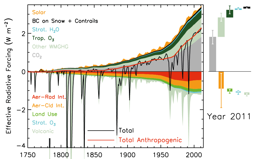
The figure from the last IPCC report below shows the various forcings of the climate system. These estimates suggest that the cooling of aerosols and the warming of greenhouse gases is similar in climate models until 1900. However, with less influence of aerosols, the warming would start earlier.

Stevens (2015) argues that we have overestimated the importance of aerosols. I do not find Stevens' arguments particularly convincing, but everyone in the field agrees that there are at least huge uncertainties. The CMIP5 figure gives the error bars at the right and it is within the confidence interval that there is effectively nearly no net influence of aerosols (ochre bar at the right).

There is direct cooling of aerosols due to scattering of solar radiation. This is indicated in red as "Aer-Rad int." This is uncertain because we do not have good estimates on the amount and size of the aerosols. Even larger uncertainties are in how aerosols influence the radiative properties of clouds, marked in ochre as "Aer-Cld int."

Some of the warming in our period was also due to less natural volcanic aerosols at the end. Their influence on climate is also uncertain because of lack of observations on the size of the eruptions and the spatial pattern of the aerosols.


Forcing estimate for the IPPC AR5 report.

The article mentioned in the beginning (Jones et al. 2013) showing the CMIP5 global climate model ensemble temperatures for all forcings, which did not show much warming in our period, also gives results for model runs that only include greenhouse gases, which shows a warming of about 0.2°C; see below. If we interpret this difference as the influence of aerosols, (there is also a natural part) then aerosols would be responsible for 0.2°C cooling in our period in the current model runs. In the limit of the confidence interval were aerosols do not have a net influence, an additional warming of 0.2°C could thus be explained by aerosols.


CMIP5 climate model ensemble (yellow lines) and its mean (red line) plotted together with several instrumental temperature estimates (black lines). Figure from Jones et al. (2013) with our box added to estimate the temperature increase.

Conclusion on early global warming

Several lines of evidence suggest that the Earth’s surface actually was warming during this period. Every line of evidence by itself is currently not compelling, but the [[consilience]] of evidence at least makes a good case for further research and especially to revisit the warming bias of early instrumental observations.

To make a good case, one would have to make sure that all datasets cover the same regions/locations. With the modest warming during this period, the analysis should be very careful. It would also need an expert for each of the different measurement types to understand the uncertainties in their trends. Anyone interested in make a real publishable study out of this please contact me.


Austrian Hann screen (a large screen build close to a northern wall) and a Stevenson screen in Graz, Austria.

Collaboration on studying the bias

To study the transition to Stevenson screens, we are collecting data from parallel measurements of early instrumentation with Stevenson screens.

We have located the data for the first seven sources listed below.

Australia, Adelaide, Glaisher stand
Austria, Kremsmünster, North Wall
Austria, Hann screen in Vienna and Graz
Spain, SCREEN project, Montsouris (French) screen in Murcia and La Coruña
Switzerland, Wild screen in Basel and Zurich
Northern Ireland, North wall in Armagh
Norway, North wall


Most are historical datasets, but there are also two modern experiments with historical screens (Spain and Kremsmünster). Such experiments with replicas is something I hope will be done more in future. It could also be an interesting project for an enthusiastic weather observer with an interest in history.

From the literature we know of a number of further parallel measurements all over the world; listed below. If you have contacts to people who may know where these datasets are, please let us know.

Belgium, Uccle, open screen
Denmark, Bovbjerg Fyr, Skjoldnñs, Keldsnor, Rudkùbing, Spodsbjerg Fyr, Gedser Fyr, North wall.
France, Paris, Montsouris (French) screen
Germany, Hohenpeissenberg, North wall
Germany, Berlin, Montsouris screen
Iceland, 8 stations, North wall
Northern Ireland, a thermograph in North wall screen in Valentia
Norway, Fredriksberg observatory, Glomfjord, Dombas, North wall
Samoa, tropic screen
South Africa, Window screen, French and Stevenson screens
Sweden, Karlstadt, Free standing shelter
Sweden, Stockholm Observatory
UK, Strathfield Turgiss, Lawson stand
UK, Greenwich, London, Glaisher stand
UK, Croydon, Glaisher stand
UK, London, Glaisher stand


To get a good estimate of the bias we need many parallel measurements, from as many early screens as possible and from many different climatic regions, especially continental, tropical and sub-tropical climates. Measurements made outside of Europe are lacking most and would be extremely valuable.

If you know of any further parallel measurements, please get in touch. It does not have to be a dataset, also a literature reference is a great hint and a starting point for a search. If your twitter followers or facebook friends may have parallel datasets please post this post on POST.


Related reading

Scientists clarify starting point for human-caused climate change

Parallel Observations Science Team (POST) of the International Surface Temperature Initiative (ISTI).

The transition to automatic weather stations. We’d better study it now.

Why raw temperatures show too little global warming.

Changes in screen design leading to temperature trend biases.

Notes


1) The difference in Basel is nearly zero if you use the local way to compute the mean temperature from fixed hour measurements, but it is about 0.25°C if you use the maximum and minimum temperature, which is mostly used in climatology.

2) Note that GHCNv3 only homogenizes the annual means, that is, every month gets the same corrections. Thus the difference in trends between summer and winter shown in the figure is like it is in the raw data.

3) The winter trend is 1.5 times the summer trend in the mean temperature of the CMIP5 ensemble for the Northern Hemisphere (ocean and land). The factor three we found in for GHCN was only for land. Thus a more careful analysis may find somewhat different values.


References

Auchmann, R. and S. Brönnimann, 2012: A physics-based correction model for homogenizing sub-daily temperature series. Journal Geophysical Research Atmospheres., 117, art. no. D17119, doi: 10.1029/2012JD018067.

Bjorn Stevens, 2015: Rethinking the Lower Bound on Aerosol Radiative Forcing. Journal of Climate, 28, pp. 4794–4819, doi: 10.1175/JCLI-D-14-00656.1.

Böhm, R., P.D. Jones, J. Hiebl, D. Frank, et al., 2010: The early instrumental warm-bias: a solution for long central European temperature series 1760–2007. Climatic Change, 101, pp. 41–67, doi: 10.1007/s10584-009-9649-4.

Brunet, M., J. Asin, J. Sigró, M. Bañón, F. García, E. Aguilar, J. Esteban Palenzuela, T.C. Peterson, P. Jones, 2011: The minimization of the screen bias from ancient Western Mediterranean air temperature records: an exploratory statistical analysis. International Journal Climatololgy, 31, 1879–1895, doi: 10.1002/joc.2192.

Jones, G. S., P. A. Stott, and N. Christidis, 2013: Attribution of observed historical near‒surface temperature variations to anthropogenic and natural causes using CMIP5 simulations. Journal Geophysical Research Atmospheres, 118, 4001–4024, doi: 10.1002/jgrd.50239.

Magnuson, John J., Dale M. Robertson, Barbara J. Benson, Randolf H. Wynne, David M. Livingstone, Tadashi Arai, Raymond A. Assel, Roger B. Barry, Virginia Card, Esko Kuusisto, Nick G. Granin, Terry D. Prowse, Kenton M. Stewart, and Valery S. Vuglinski, 2000: Historical trends in lake and river ice cover in the Northern Hemisphere. Science, 289, pp. 1743-1746, doi: 10.1126/science.289.5485.1743

Nicholls, N., R. Tapp, K. Burrows, and D. Richards, 1996: Historical thermometer exposures in Australia. International Journal of Climatology, 16, pp. 705-710, doi: 10.1002/(SICI)1097-0088(199606)16:6<705::AID-JOC30>3.0.CO;2-S.

Oerlemans, J., 2005: Extracting a Climate Signal from 169 Glacier Records. Science, 308, no. 5722, pp. 675-677, doi: 10.1126/science.1107046.

Parker, D.E., 1994: Effects of changing exposure of thermometers at land stations. International Journal Climatology, 14, pp. 1–31, doi: 10.1002/joc.3370140102.

Photo at the top a Stevenson screen of the amateur weather station near Czarny Dunajec, Poland. Photographer: Arnold Jakubczyk.
Photos of Wild screen and Stevenson screen in Basel by Paul Della Marta.
Photo of open shelter in Belgium by Belgium weather service.
Photo of French screen in Spain courtesy of SCREEN project.
Photo of Hann screen and Stevenson screen in Graz courtesy of the University of Graz.

Saturday, January 16, 2016

The transition to automatic weather stations. We’d better study it now.

This is a POST post.

The Parallel Observations Science Team (POST) is looking across the world for climate records which simultaneously measure temperature, precipitation and other climate variables with a conventional sensor (for example, a thermometer) and modern automatic equipment. You may wonder why we take the painstaking effort of locating and studying these records. The answer is easy: the transition from manual to automated records has an effect on climate series and the analysis we do over them.

In the last decades we have seen a major transition of the climate monitoring networks from conventional manual observations to automatic weather stations. It is recommended to compare these instruments before the substitution is effective with side by side measurements, which we call parallel measurements. Climatologists have also set up many longer experimental parallel measurements. They tell us that in most cases both sensors do not measure the same temperature or collect the same amount of precipitation. A different temperature is not only due to the change of the sensor itself, but automatic weather stations also often use a different, much smaller, screen to protect the sensor from the sun and the weather. Often the introduction of automatic weather stations is accompanied by a change in location and siting quality.

From studies of single temperature networks that made such a transition we know that it can cause large jumps; the observed temperatures at a station can go up or down by as much as 1°C. Thus potentially this transition can bias temperature trends considerably. We are now trying to build a global dataset with parallel measurements to be able to quantify how much the transition to automatic weather stations influences the global mean temperature estimates used to study global warming.

Temperature

This study is led by Enric Aguilar and the preliminary results below were presented at the Data Management Workshop in Saint Gallen, Switzerland last November. We are still in the process of building up our dataset. Up to now we have data from 10 countries: Argentina (9 pairs), Australia (13), Brazil (4), Israel (5), Kyrgyzstan (1), Peru (31), Slovenia (3), Spain (46), Sweden (8), USA (6); see map below.


Global map in which we only display the 10 countries for which we have data. The left map is for the maximum temperature (TX) and the right for the minimum temperature (TN). Blue dots mean that the automatic weather station (AWS) measures cooler temperatures than the conventional observation, red dots mean the AWS is warmer. The size indicates how large the difference is, open circles are for statistically not significant differences.

The impact of the automation can be better assessed in the box plots below.


The bias of the individual pairs are shown as dots and summarized per country with box plots. For countries with only a few pairs the boxplots should be taken with a grain of salt. Negative values mean that the automatic weather stations are cooler. We have data for Argentina (AR), Australia (AU), Brazil (BR), Spain (ES), Israel (IL), Kyrgyzstan (KG), Peru (PE), Sweden (SE), Slovenia (SI) and the USA (US). Panels show the maximum temperature (TX), minimum temperature (TN), mean temperature (TM) and Diurnal temperature range (DTR, TX-TN).

On average there are no real biases in this dataset. However, if you remove Peru (PE) the differences in the mean temperature are either small or negative. That one country is so important shows that our dataset is currently too small.

To interpret the results we need to look at the main causes for the differences. Important reasons are that Stevenson screens can heat up in the sun on calm days, while automatic sensors are sometimes ventilated. The automatic sensors are, furthermore, typically smaller and thus less affected by direct radiation hitting them than thermometers. On the other hand, in case of conventional observation, the maintenance of the Stevenson screens—cleaning and painting—and detection of other problems may be easier because they have to be visited daily. There are concerns that plastic screens get more grey and heat more in the sun. Stevenson screens have more thermal inertia, they smooth fast temperature fluctuations, and will thus show lower highs and higher lows.

Also the location often changes with the installation of automatic weather stations. America was one of the early adopters. The US National Weather Service installed analogue semi-automatic equipment (MMTS) that did not allow for long cables between the sensor and the display inside a building. Furthermore, the technicians only had one day per station and as a consequence many of the MMTS systems were badly sited. Nowadays technology has advanced a lot and made it easier to find good sites for weather stations. This is maybe even easier now than it used to be for manual observations because modern communication is digital and if necessary uses radio making distance much less a concern. The instruments can be powered by batteries, solar or wind, which frees them from the electricity grid. Some instruments store years of data and need just batteries.

In the analysis we thus need to consider whether the automatic sensors are placed in Stevenson screens and whether the automatic weather station is at the same location. Where the screen and the location did not change (Israel and Slovenia), the temperature jumps are small. Whether the automatic weather station reduces radiation errors by mechanical ventilation is likely also important. Because of these different categories, the number of datasets needed to get a good global estimate becomes larger. Up to now, these factors seem to be more important than the climate.

Precipitation

For most of these countries we also have parallel measurements for precipitation. The figure below was made by Petr Stepanek, who leads this part of the study.


Boxplots for the differences in monthly precipitation sums due to automation. Positive values mean that the manual observations record more precipitation. Countries are: Argentina (AG), Brazil (BR), The Check Republic (CZ), Israel (IS), Kyrgyzstan (KG), Peru (PE), Sweden (SN), Spain (SP) and the USA (US). The width of the boxplots corresponds to the size of the given dataset.

For most countries the automatic weather stations record less precipitation. This is mainly due to smaller amounts of snow during the winter. Observers often put a snow cross in the gauge in winter to make it harder for snow to blow out of it again. Observers simply melt the snow gathered in a pot to measure precipitation, while early automatic weather stations did not work well with snow and sticky snow piling up in the gauge may not be noticed. These problems can be solved by heating the gauge, but unfortunately the heater can also increase the amount of precipitation that evaporates before it could be registered. Such problems are known and more modern rain gauges use different designs and likely have a smaller bias again.

Database with parallel data

The above results are very preliminary, but we wanted to show the promise of a global dataset with parallel data to study biases in the climate record due to changes in the observing practises. To proceed we need more datasets and better information on how the measurements were performed to make this study more solid.

In future we also want to look more at how the variability around the mean is changing. We expect that changes in monitoring practices have a strong influence on the tails of the distribution and thus on estimates of changes in extreme weather. Parallel data offer a unique opportunity to study this otherwise hard problem.

Most of the current data comes from Europe and South America. If you know of any parallel datasets especially from Africa or Asia, please let us know. Up to now, the main difficulty for this study is to find the persons who know where the data is. Fortunately, data policies do not seem to be a problem. Parallel data is mostly seen as experimental data. In some cases we “only” got a few years of data from a longer dataset, which would otherwise be seen as operational data.

We would like to publish the dataset after publishing our papers about it. Again this does not seem to lead to larger problems; sometimes people prefer to first publish an article themselves, which causes some delays, and sometimes we cannot publish the daily data itself, but “only” monthly averages and extreme value indices, this makes the results less transparent, but these summary values contain most of the information.

Knowledge of the observing practices is very important in the analysis. Thus everyone who contributes data is invited to help in the analysis of the data and co-author our first paper(s). Our studies are focused on global results, but we will also provide everyone with results for their own dataset to gain a better insight into their data.

Most climate scientists would agree that it is important to understand the impact of automation on our records. So does the World Meteorological Organization. In case it helps you to convince your boss: the Parallel Observations Science Team is part of the International Surface Temperature Initiative (ISTI). It is endorsed by the Task Team on Homogenization (TT-HOM) of the World Meteorological Organization (WMO).

We expect that this endorsement and our efforts to raise awareness about our goals and their importance will help us to locate and study parallel observations from other parts of the world, especially Africa and Asia. We also expect to be able to get more data from Europe; the regional association for Europe of the WMO has designated the transition to automatic weather stations as one of its priorities and is helping us to get access to more data. We want to have datasets for all over the world to be able to assess whether the station settings (sensors, screens, data quality, etc.) have an impact, but also to understand if different climates produce different biases.

If you would like to collaborate or have information, please contact me.


Related reading

The ISTI has made a series of brochures on POST in English, Spanish, French and German. If anyone is able to make further translations, that would be highly appreciated.

Parallel Observations Science Team of the International Surface Temperature Initiative.

Irrigation and paint as reasons for a cooling bias

Temperature trend biases due to urbanization and siting quality changes

Changes in screen design leading to temperature trend biases

Temperature bias from the village heat island

Sunday, October 4, 2015

Measuring extreme temperatures in Uccle, Belgium


Open thermometer shelter with a single set of louvres.

That changes in the measurement conditions can lead to changes in the mean temperature is hopefully known by most people interested in climate change by now. That such changes are likely even more important when it comes to weather variability and extremes is unfortunately less known. The topic is studied much too little given its importance for the study of climatic changes in extremes, which are expected to be responsible for a large part of the impacts from climate change.

Thus I was enthusiastic when a Dutch colleague send me a news article on the topic from the homepage of the Belgium weather service, Koninklijk Meteorologisch Instituut (KMI). It describes a comparison of two different measurement set-ups, old and new, made side by side in [[Uccle]], the main office of the KMI. The main difference is the screen used to protect the thermometer from the sun. In the past these were often more open, that makes ventilation better, nowadays they are more closed to reduce (solar and infra red) radiation errors.

The more closed screen is a [[Stevenson screen]], invented in the last decades of the 19th century. I had assumed that most countries had switched to Stevenson screens before the 1920s. But I recently learned that Switzerland changed in the 1960s and in Uccle they changed in 1983. Making any change to the measurements is a difficult trade off between improving the system and breaking the homogeneity of the climate record. It would be great to have a historical overview of such historical transitions in the way climate is measured for all countries.

I am grateful to the KMI for their permission to republish the story here. The translation, clarifications between square brackets and the related reading section are mine.


Closed thermometer screen with a double-louvred walls [Stevenson screen].
In the [Belgian] media one reads regularly that the highest temperature in Belgium is 38.8°C and that it was recorded in Uccle on June 27, 1947. Sometimes, one also mentions that the measurement was conducted in an "open" thermometer screen. On warm days the question typically arises whether this record could be broken. In order to be able to respond to this, it is necessary to take some facts into account that we will summarize below.

It is important to know that temperature measurements are affected by various factors, the most important one is the type of the thermometer screen in which the observations are carried out. One wants to measure the air temperature and therefore prevent a warming of the measuring equipment by protecting the instruments from the distorting effects of solar radiation. The type of thermometer screen is particularly important on sunny days and this is reflected in the observations.

Since 1983, the reference measurements of the weather station Uccle are made in a completely "closed" thermometer screen [a Stevenson screen] with double-louvred walls. Until May 2006, the reference thermometers were mercury thermometers for daily maximums and alcohol thermometers for daily minimums. [A typical combination nowadays because mercury freezes at -38.8°C.] Since June 2006, the temperature measurements are carried out continuously by means of an automatic sensor in the same type of closed cabin.

Before 1983, the measurements were carried out in an "open" thermometer screen with only a single set of louvres, which on top of that offered no protection on the north side. Because of the reasons mentioned above, the maximum temperature in this type of shelter were too high, especially during the summer period with intense sunshine. On July 19, 2006, one of the hottest days in Uccle, for example, the reference [Stevenson] screen measured a maximum temperature of 36.2°C compared to 38.2°C in the "open" shelter on the same day.

As the air temperature measurements in the closed screen are more relevant, it is advisable to study the temperature records that would be or have been measured in this type of reference screen. Recently we have therefore adjusted the temperature measurements of the open shelter from before 1983, to make them comparable with the values from the closed screen. These adjustments were derived from the comparison between the simultaneous [parallel] observations measured in the two types of screens during a period of 20 years (1986-2005). Today we therefore have two long series of daily temperature extremes (minimum and maximum), beginning in 1901, corresponding to measurements from a closed screen.

When one uses the alignment method described above, the estimated value of the maximum temperature in a closed screen on June 27, 1947, is 36.6°C (while a maximum value of 38.8°C was measured in an open screen, as mentioned in the introduction). This value of 36.6°C should therefore be recognized as the record value for Uccle, in accordance with the current measurement procedures. [For comparison, David Parker (1994) estimated that the cooling from the introduction of Stevenson screens was less than 0.2°C in the annual means in North-West Europe.]

For the specialists, we note that the daily maximum temperature shown in the synoptic reports of Uccle, usually are up to a few tenths of a degree higher compared with the reference climatological observations that were mentioned previously. This difference can be explained by the time intervals over which the temperature is averaged in order to reduce the influence of atmospheric turbulence. The climatic extremes are calculated over a period of ten minutes, while the synoptic extremes are calculated from values ​​that were averaged over a time span of a minute. In the future, will make these calculation methods the same by applying the climatic procedures always.

Related reading

KMI: Het meten van de extreme temperaturen te Ukkel

To study the influence of such transitions in the way the climate is measured using parallel data we have started the Parallel Observations Science Team (ISTI-POST). One of the POST studies is on the transition to Stevenson screens, which is headed by Theo Brandsma. If you have such data please contact us. If you know someone who might, please tell them about POST.

Another parallel measurement showing huge changes in the extremes is discussed in my post: Be careful with the new daily temperature dataset from Berkeley

More on POST: A database with daily climate data for more reliable studies of changes in extreme weather

Introduction to series on weather variability and extreme events

On the importance of changes in weather variability for changes in extremes

A research program on daily data: HUME: Homogenisation, Uncertainty Measures and Extreme weather

Reference

Parker, David E., 1994: Effect of changing exposure of thermometers at land stations. International journal of climatology, 14, pp. 1-31, doi: 10.1002/joc.3370140102.

Tuesday, June 9, 2015

Comparing the United States COOP stations with the US Climate Reference Network

Last week the mitigation sceptics apparently expected climate data to be highly reliable and were complaining that an update led to small changes. Other weeks they expect climate data to be largely wrong, for example due to non-ideal micro-siting or urbanization. These concerns can be ruled out for the climate-quality US Climate Reference Network (USCRN). This is a guest post by Jared Rennie* introducing a recent study comparing USCRN stations with nearby stations of the historical network, to study the differences in the temperature and precipitation measurements.


Figure 1. These pictures show some of instruments from the observing systems in the study. The exterior of a COOP cotton region shelter housing a liquid-in-glass thermometer is pictured in the foreground of the top left panel, and a COOP standard 8-inch precipitation gauge is pictured in the top right. Three USCRN Met One fan-aspirated shields with platinum resistance thermometers are pictured in the middle. And, a USCRN well-shielded Geonor weighing precipitation gauge is pictured at the bottom.
In 2000 the United States started building a measurement network to monitor climate change, the so called United States Climate Reference Network (USCRN). These automatic stations have been installed in excellent locations and are expected not to show influences of changes in the direct surroundings for decades to come. To avoid loss of data the most important variables are measured by three high-quality instruments. A new paper by Leeper, Rennie, and Palecki now compares the measurements of twelve station pairs of this reference network with nearby stations of the historical US network. They find that the reference network records slightly cooler temperature and less precipitation and that there are almost no differences in the temperature variability and trend.

COOP and USCRN

The detection and attribution of climate signals often rely upon long, historically rich records. In the United States, the Cooperative Observer Program (COOP) has collected many decades of observations for thousands of stations, going as far back as the late 1800’s. While the COOP network has become the backbone of the U.S. climatology dataset, non-climatic factors in the data have introduced systematic biases, which require homogenization corrections before they can be included in climatic assessments. Such factors include modernization of equipment, time of observation differences, changes in observing practices, and station moves over time. A part of the COOP stations with long observations is known as the US Historical Climate Network (USHCN), which is the default dataset to report on temperature changes in the USA.

Recognizing these challenges, the United States Climate Reference Network (USCRN) was initiated in 2000. 15 years after its inception, 132 stations have been installed across the United States with sub-hourly observations of numerous weather elements using state-of-the-art instrumentation calibrated to traceable standards. For a high data quality temperature and precipitation sensors are well shielded and for continuity the stations have three independent sensors, so no data loss is incurred. Because of these advances, no homogenization correction is necessary.

Comparison

The purpose of this study is to compare observations of temperature and precipitation from closely spaced members of USCRN and COOP networks. While the pairs of stations are near to each other they are not adjacent. Determining the variations in data between the networks allows scientists to develop an improved understanding of the quality of weather and climate data, particularly over time as the periods of overlap between the two networks lengthen.

To ensure observational differences are the result of network discrepancies, comparisons were only evaluated for station pairs located within 500 meters. The twelve station pairs chosen were reasonably dispersed across the lower 48 states of the US. Images of the instruments used in both networks are provided in Figure 1.

The USCRN stations all have the same instrumentation: well-shielded rain gauges and mechanically ventilated temperature sensors. Two types of thermometers are used: modern automatic electrical sensors known as the maximum-minimum temperature sensor (MMTS ) and old-fashioned normal thermometers, which now have to be called liquid-in-glass (LiG) thermometers. Both are naturally ventilated.

An important measurement problem for rain gauges is undercatchment: due to turbulence around the instruments not all droplets land in the mouth. This is especially important in case of high winds and for snow and can be reduced by wind shields. The COOP rain gauges are unshielded, however, and have been known to underestimate precipitation in windy conditions. COOP gauges also include a funnel, which can be removed before snowfall events. The funnel reduces evaporation losses on hot days, but can also get clogged by snow. Hourly temperature data from USCRN were averaged into 24 hour periods to match daily COOP measurements at the designated observation times, which vary by station. Precipitation data was aggregated into precipitation events and also matched with respective COOP events.

Observed differences and their reasons

Overall, COOP sensors in shields naturally ventilated reported warmer daily maximum temperatures (+0.48°C) and cooler daily minimum temperatures (-0.36°C) than USCRN sensors, which have better solar shielding and fans to ventilate the instrument. The magnitude of temperature differences were on average larger for stations operating LiG systems, than those for the MMTS system. Part of the reduction in network biases with the MMTS system is likely due to the smaller-sized shielding that requires less surface wind speed to be adequately ventilated.

While overall mean differences were in line with side-by-side comparisons of ventilated and non-ventilated sensors, there was considerable variability in the differences from station to station (see Figure 2). While all COOP stations observed warmer maximum temperatures, not all saw cooler minimum temperatures. This may be explained by differing meteorological conditions (surface wind speed, cloudiness), local siting (heat sources and sinks), and sensor and human errors (poor calibration, varying observation time, reporting error). While all are important to consider, meteorological conditions were only examined further by categorizing temperature differences by wind speed. The range in network differences for maximum and minimum temperatures seemed to reduce with increasing wind speed, although more so with maximum temperature, as sensor shielding becomes better ventilated with increasing wind speed. Minimum temperatures are highly driven by local radiative and siting characteristics. Under calm conditions one might expect radiative imbalances between naturally and mechanically aspirated shields or differing COOP sensors (LiG vs MMTS). That along with local vegetation and elevation differences may help to drive these minimum temperature differences.


Figure 2. USCRN minus COOP average minimum (blue) and maximum (red) temperature differences for collocated station pairs. COOP stations monitoring temperature with LiG technology are denoted with asterisks.

For precipitation, COOP stations reported slightly more precipitation overall (1.5%). Similar to temperature, this notion was not uniform across all station pairs. Comparing by season, COOP reported less precipitation than USCRN during winter months and more precipitation in the summer months. The dryer wintertime COOP observations are likely due to the lack of gauge shielding, but may also be impacted by the added complexity of observing solid precipitation. An example is removing the gauge funnel before a snowfall event and then melting the snow to calculate liquid equivalent snowfall.

Wetter COOP observations over warmer months may have been associated with seasonal changes in gauge biases. For instance, observation errors related to gauge evaporation and wetting factor are more pronounced in warmer conditions. Because of its design, the USCRN rain gauge is more prone to wetting errors (that some precipitation sticks to the wall and is thus not counted). In addition, USCRN does not use an evaporative suppressant to limit gauge evaporation during the summer, which is not an issue for the funnel-capped COOP gauge. The combination of elevated biases for USCRN through a larger wetting factor and enhanced evaporation could explain wetter COOP observations. Another reason could be the spatial variability of convective activity. During summer months, daytime convection can trigger unorganized thundershowers whose scale is small enough where it would report at one station, but not another. For example, in Gaylord Michigan, the COOP observer reported 20.1 mm more than the USCRN gauge 133 meters away. Rain radar estimates showed nearby convection over the COOP station, but not the USCRN, thus creating a valid COOP observation.


Figure 3. Event (USCRN minus COOP) precipitation differences grouped by prevailing meteorological conditions during events observed at the USCRN station. (a) event mean temperature: warm (more than 5°C), near-freezing (between 0°C and 5°C), and freezing conditions (less than 0°C); (b) event mean surface wind speed: light (less than 1.5 m/s), moderate (between 1.5 m/s and 4.6 m/s), and strong (larger than 4.6 m/s); and (c) event precipitation rate: low (less than 1.5 mm/hr), moderate (between 1.5 mm/hr and 2.8 mm/hr), and intense (more than 2.8 mm/hr).

Investigating further, precipitation events were categorized by air temperature, wind speed, and precipitation intensity (Figure 3). Comparing by temperature, results were consistent with the seasonal analysis, showing lower COOP values (higher USCRN) in freezing conditions and warmer COOP values (lower USCRN) in near-freezing and warmer conditions. Stratifying by wind conditions is also consistent, indicating that the unshielded gauges in COOP will not catch as much precipitation as it should, showing a higher USCRN value. On the other hand, COOP reports much more precipitation in lighter wind conditions, due to higher evaporation rate in the USCRN gauge. For precipitation intensity, USCRN observed less than COOP for all categories.


Figure 4. National temperature anomalies for maximum (a) and minimum (b) temperature between homogenized COOP data from the United States Historical Climatology Network (USHCN) version 2.5 (red) and USCRN (blue).
Comparing the variability and trends between USCRN and homogenized COOP data from USHCN we see that they are very similar for both maximum and minimum national temperatures (Figure 4).

Conclusions

This study compared two observing networks that will be used in future climate and weather studies. Using very different approaches in measurement technologies, shielding, and operational procedures, the two networks provided contrasting perspectives of daily maximum and minimum temperatures and precipitation.

Temperature comparisons between stations in local pairings were partially attributed to local factors including siting (station exposure), ground cover, and geographical aspects (not fully explored in this study). These additional factors are thought to accentuate or minimize anticipated radiative imbalances between the naturally and mechanically aspirated systems, which may have also resulted in seasonal trends. Additional analysis with more station pairs may be useful in evaluating the relative contribution of each local factor noted.

For precipitation, network differences also varied due to the seasonality of the respective gauge biases. Stratifying by temperature, wind speed, and precipitation intensity showed these biases are revealed in more detail. COOP gauges recorded more precipitation in warmer conditions with light winds, where local summertime convection and evaporation in USCRN gauges may be a factor. On the other hand, COOP recorded less precipitation in colder, windier conditions, possibly due to observing error and lack of shielding, respectively.

It should be noted that all observing systems have observational challenges and advantages. The COOP network has many decades of observations from thousands of stations, but it lacks consistency in instrumentation type and observation time in addition to instrumentation biases. USCRN is very consistent in time and by sensor type, but as a new network it has a much shorter station record with sparsely located stations. While observational differences between these two separate networks are to be expected, it may be possible to leverage the observational advantages of both networks. The use of USCRN as a reference network (consistency check) with COOP, along with more parallel measurements, may prove to be particularly useful in daily homogenization efforts in addition to an improved understanding of weather and climate over time.


* Jared Rennie currently works at the Cooperative Institute for Climate and Satellites – North Carolina (CICS-NC), housed within the National Oceanic and Atmospheric Administration’s (NOAA’s) National Centers for Environmental Information (NCEI), formerly known as the National Climatic Data Center (NCDC). He received his masters and bachelor degrees in Meteorology from Plymouth State University in New Hampshire, USA, and currently works on maintaining and analyzing global land surface datasets, including the Global Historical Climatology Network (GHCN) and the International Surface Temperature Initiative’s (ISTI) Databank.

Further reading

Ronald D. Leeper, Jared Rennie, and Michael A. Palecki, 2015: Observational Perspectives from U.S. Climate Reference Network (USCRN) and Cooperative Observer Program (COOP) Network: Temperature and Precipitation Comparison. Journal Atmospheric and Oceanic Technology, 32, pp. 703–721, doi: 10.1175/JTECH-D-14-00172.1.

The informative homepage of the U.S. Climate Reference Network gives a nice overview.

A database with parallel climate measurements, which we are building to study the influence of instrumental changes on the probability distributions (extreme weather and weather variability changes).

The post, A database with daily climate data for more reliable studies of changes in extreme weather, provides a bit more background on this project.

Homogenization of monthly and annual data from surface stations. A short description of the causes of inhomogeneities in climate data (non-climatic variability) and how to remove it using the relative homogenization approach.

Previously I already had a look at trend differences between USCRN and USHCN: Is the US historical network temperature trend too strong?